Building an HNSW Index From Scratch In C++ (1/2)

Vishvam Mar 5, 2026 15 min read

c++ machine-learning algorithms exploratory

Introduction

Even before moving on to what an HNSW index is, let’s first look at the problem at hand : we have a document and we want to check which other documents are similar to it. There are many ways to solve this problem. One approach is to do a “keyword”-based count and evaluate how many overlaps there are. This works well for documents requiring precise information, like legal documents. But this approach doesn’t capture the semantic meaning of a document. So, performing natural language queries like “Which division has the highest profits?” or “How many paid time-offs are available per year?” becomes difficult.

To capture semantics, we use embeddings. Embeddings are vectors of fixed length. For example, the query “Which division has the highest profits?” is first split into tokens: [12, 34, 123, 534, 32, 435]. Each token is then converted into a vector of fixed size :

112 -> [0.12, -0.88, 0.44, ..., 0.01]
234 -> [-0.34, 0.91, 0.11, ..., -0.55]
3...

There are many ways to generate embeddings, but to stay close to the topic, I won’t go into that here.

But What’s HSN .. HNS .. HWS … HSNW … HNSW 😭

When building RAG (Retrieval-Augmented Generation) applications, you often need to store and query embeddings of documents efficiently. Libraries like FAISS, Pinecone, and Milvus provide this functionality by implementing Approximate Nearest Neighbor (ANN) search algorithms.

Different libraries use different approaches to store embeddings to make ANN search efficient. Broadly, these approaches can be grouped into three categories :

Tree-based methods: Organize vectors hierarchically. Examples include k-d trees and ball trees.
Hashing-based methods: Map similar vectors to the same “bucket” to enable fast lookup. A common technique is Locality-Sensitive Hashing (LSH).
Graph-based methods : Connect vectors in a proximity graph, where closer vectors are linked together

As Pinecone explains:

“We can split ANN algorithms into three distinct categories: trees, hashes, and graphs. HNSW slots into the graph category. More specifically, it is a proximity graph, in which two vertices are linked based on their proximity — often defined using Euclidean distance.”

Why HNSW?

HNSW — Hierarchical Navigable Small World graphs is a graph-based data structure designed for efficient ANN search in high-dimensional spaces. Instead of comparing a query vector against every vector in the dataset (brute-force search, O(N) complexity), HNSW organizes vectors into multiple layers of proximity graphs.

This design enables sub-linear search times in practice (usually O(logN)), making it ideal for large-scale vector datasets. Many modern vector databases rely on HNSW under the hood, including:

By leveraging HNSW, these systems can efficiently retrieve nearest neighbours even in very large datasets, which is crucial for embedding-based search and RAG applications.

Sounds Good. How Does It Work ?

HNSW is a graph with embeddings as nodes. So, something like this :

 1#include <vector>
 2
 3using std::vector;
 4
 5class Node {
 6public:
 7    int id;
 8    vector<float> embedding;
 9    vector<vector<int>> neighbours;
10
11    Node(int id, const vector<float>& embedding);
12};

At least in my experience, whenever there is a O(N) to O(logN) dip, I think of something related to trees / layers / binary search / etc. In this case too, we have a “layer” based implementation which helps decrease the time complexity.

The main idea behind HNSW is, we will have at most M layers … layer M being the top-most and layer 0 being the bottom-most layer. The top-most layer is very sparse and the bottom-most layer is very dense. One of the nodes at the top-most layer is the “entry point”. Meaning, whenever we want to start our search, we start FROM the entry point

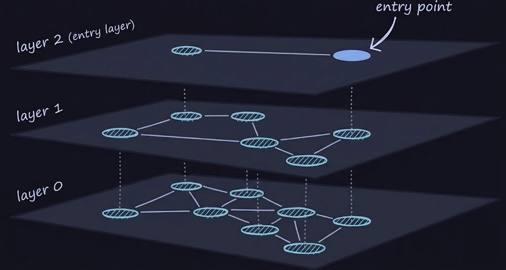
HNSW graph (istg the name 😭 anyhow, click to enlarge)

From the above diagram, the search procedure might be a bit more clear now. We start from the entry point, search its neighbours, go down, search its neighbours, go down and so on. But, you may ask kindly, “how the heck is that O(logN) … aren’t we traversing the whole graph ?” and answer to that is yes … we are. But while searching, we don’t explore all the neighbours. We pick the N closest ones per layer and proceed with those (In the actual paper, N is referred to as efSearch … ef, if I’m not mistaken stands for exploration factor)

How Do We Model Layers Now ?

As with any problem in computer science, there are multiple ways to do this. One can encode the level information in the edges of the graph or perhaps can maintain a map of layer -> node. For the sake of simplicity, I just encode that in the Node itself :

 1#include <vector>
 2
 3using std::vector;
 4
 5class Node {
 6public:
 7    int id;
 8    int level;
 9    vector<float> embedding;
10    vector<vector<int>> neighbours;
11
12    Node(int id, int level, const vector<float>& embedding);
13};

So, layers / levels is accommodated. We now need to figure out a way to add and search elements. I’ll be following these declarations :

 1class HnswIndex {
 2public:
 3    virtual ~HnswIndex() = default;
 4
 5	// For adding embeddings to our graph
 6    virtual void create(const vector<vector<float>>& data) = 0;
 7    virtual void add(const vector<float>& embedding) = 0;
 8
 9	// ANN search
10    virtual vector<int> search(const vector<float>& query, int k, int efSearch = 50) = 0;
11
12	// Just a util
13	virtual int size() const = 0;
14};

And these will the inner details of the HnswCPU class (this contains the parameters, graph representation, etc) :

 1class HnswCPU : public HnswIndex {
 2  private:
 3    int M;
 4    int M0;
 5    int efConstruction;
 6    double levelMultiplier;
 7
 8	// Graph internals
 9    vector<Node> nodes;
10    int entryPoint;
11    int maxLevel;
12    int currentId;
13
14	// Random number generators ... c++ ik
15    std::mt19937 gen;
16    std::uniform_real_distribution<float> uniform_dist;
17
18    DistanceType distType;
19    DistFunc distFunc;
20
21    int sampleLevel();
22    double l2Distance(const vector<float> &a, const vector<float> &b) const;
23
24	// Utility methods
25    vector<int> searchLayer(
26		const vector<float> &query,
27		int entry, int ef, int level
28	);
29
30    vector<int> selectneighbours(
31        const vector<float> &query,
32        const vector<int> &candidates,
33        int max_neighbours
34    );
35
36	// Will discuss this soon
37    vector<int> selectneighboursWithHeuristic(
38        const vector<float> &query,
39        const vector<int> &candidates,
40        int max_neighbours,
41        int layer,
42        bool extendCandidates,
43        bool keepPrunedConnections
44    );
45
46  public:
47    HnswCPU(
48        int M = 16,
49        int efConstruction = 200,
50        uint32_t seed = 42,
51        DistanceType distType = DistanceType::L2,
52
53		// Ignore this for now. In Part 2, we'll explore SIMD and we will see how
54		// it compares to non-SIMD variant (this)
55        bool forceScalar = false
56    );
57
58    void create(const vector<vector<float>> &data) override;
59    void add(const vector<float> &embedding) override;
60
61    vector<int> search(const vector<float> &query, int k, int efSearch = 50) override;
62
63	// Again, ignore
64	int size() const override;
65
66    void printInfo();
67
68};

Note

.... From here on, there is gonna a ton of code snippets. Please bear with me 🫠

Implementing The Utility Methods First

`SearchLayer` Procedure

This method takes in a layer, an entrypoint in that layer and returns the top-K closest nodes in a layer where

1K = min(ef, number_of_nodes_reached_during_search)

Here's where cool data structures like heaps come into picture.

First, like any other graph traversal problem, we push the entry node and the initial distance (= 0) on to the min-heap, then start the exploration.

Second, we also need the top-k closest nodes. Inorder to compute that, we will use a max-heap and keep track of distances of nodes in this order : farthest -> ... -> closest and yoink the root element if the size of the max-heap becomes greater than the exploration factor (ef)

The implementation looks something like this :

 1vector<int> HnswCPU::searchLayer(
 2    const vector<float> &query, int entry, int ef, int level
 3) {
 4
 5    using DistanceIndexPair = pair<double, int>;
 6
 7    // Min heap
 8    priority_queue<
 9        DistanceIndexPair,
10        vector<DistanceIndexPair>,
11        std::greater<>
12    > candidates;
13
14    // Max heap
15    priority_queue<DistanceIndexPair> topResults;
16
17    vector<uint8_t> visited(nodes.size(), 0);
18
19    double dist = l2Distance(query, nodes[entry].embedding);
20
21    candidates.push({dist, entry});
22    topResults.push({dist, entry});
23    visited[entry] = 1;
24
25    while (!candidates.empty()) {
26
27        auto [currDist, currId] = candidates.top();
28        candidates.pop();
29
30        if (currDist > topResults.top().first)
31            break;
32
33        for (int nei : nodes[currId].neighbours[level]) {
34
35            if (visited[nei])
36                continue;
37
38            visited[nei] = 1;
39
40            double d = l2Distance(query, nodes[nei].embedding);
41
42            if (static_cast<int>(topResults.size()) < ef ||
43                d < topResults.top().first) {
44
45                candidates.push({d, nei});
46                topResults.push({d, nei});
47
48                if (static_cast<int>(topResults.size()) > ef)
49                    topResults.pop();
50            }
51        }
52    }
53
54    vector<int> result;
55    while (!topResults.empty()) {
56        result.push_back(topResults.top().second);
57        topResults.pop();
58    }
59
60    return result;
61}

Note

If you’re perceptive, you might have noticed that result actually contains the elements in reverse order. We could reverse it here, but the original paper does not reverse the results from searchLayer, so we follow that approach. Later, in selectneighbours and its variants, we include a sort step at the end to ensure the elements are in order

`SelectNeighbours` Procedure

The basic implementation is pretty straightforward. For each neighbour of a node, we just call searchLayer, sort the results and pick the top-K closest ones. The implementation looks something like this :

 1vector<int> HnswCPU::selectneighbours(
 2    const vector<float> &query,
 3    const vector<int> &candidates,
 4    int max_neighbours
 5) {
 6
 7    vector<pair<double, int>> distList;
 8
 9    for (int id : candidates) {
10        distList.emplace_back(l2Distance(query, nodes[id].embedding), id);
11    }
12
13    std::sort(distList.begin(), distList.end());
14
15    vector<int> result;
16    for (int i = 0; i < std::min(max_neighbours, static_cast<int>(distList.size()));++i) {
17        result.push_back(distList[i].second);
18    }
19
20    return result;
21}

One of the major flaws with the naive approach is that recall@k is poor. Fortunately, the original paper also proposes a heuristic based approach for selecting neighbours

Note

Recall@k measures how many true nearest neighbours you found. For example, top-10 neighbours known from brute force. Your ANN returns 10 results. 9 of them are correct. So, Recall@10=9/10=0.9

Anyhow, what the paper suggests is that when selecting neighbours, we :

Take closest candidates to the query.
Accept a candidate only if it is not closer to any already selected neighbor than to the query. Meaning, don’t connect to nodes that are redundant (too close to an already chosen one).

It forces angular diversity as it prefers nodes that are close to the query but also far from each other. So, we don't want something like this : (all clustered in the same direction)

1query ●
2   |
3   ● c1
4   ● c2
5   ● c3

That creates:

Highly redundant connections
Poor graph navigation
Local clustering
Worse long-range routing

We want something like this :

1        ● c2
2
3query ●
4
5        ● c3
6
7   ● c1

This creates:

Better navigability
Shorter greedy paths
Logarithmic search behavior

Implementation for that looks something like this :

 1vector<int> HnswCPU::selectneighboursWithHeuristic(
 2    const vector<float> &query,
 3    const vector<int> &candidates,
 4    int max_neighbours,
 5    int layer,
 6    bool extendCandidates,
 7    bool keepPrunedConnections
 8) {
 9
10    vector<int> result;
11
12    // Min heap
13    priority_queue<
14        DistanceIndexPair,
15        vector<DistanceIndexPair>,
16        std::greater<>
17    > pq;
18
19    // Max heap
20    priority_queue<
21        DistanceIndexPair,
22        vector<DistanceIndexPair>,
23        std::greater<>
24    > discarded;
25
26    vector<uint8_t> visited(nodes.size(), 0);
27
28    for (int cand : candidates) {
29
30        if (!visited[cand]) {
31            visited[cand] = 1;
32            pq.push({l2Distance(query, nodes[cand].embedding), cand});
33        }
34
35        if (extendCandidates) {
36            for (int nei : nodes[cand].neighbours[layer]) {
37                if (!visited[nei]) {
38                    visited[nei] = 1;
39                    pq.push({l2Distance(query, nodes[nei].embedding), nei});
40                }
41            }
42        }
43    }
44
45    while (!pq.empty() && static_cast<int>(result.size()) < max_neighbours) {
46
47        auto [dist, id] = pq.top();
48        pq.pop();
49
50        bool good = true;
51
52        // This enforces the "angular" diversity so to say
53        for (int r : result) {
54            if (l2Distance(nodes[id].embedding, nodes[r].embedding) < dist) {
55                good = false;
56                break;
57            }
58        }
59
60        if (good) {
61            result.push_back(id);
62        } else {
63            discarded.push({dist, id});
64        }
65    }
66
67    // Just to capture extra nodes as the search space extinguishes
68    // pretty quickly
69    if (keepPrunedConnections) {
70        while (!discarded.empty() &&
71               static_cast<int>(result.size()) < max_neighbours) {
72            result.push_back(discarded.top().second);
73            discarded.pop();
74        }
75    }
76
77    return result;
78}

Coming Back To The Actual Methods

ANN `Search` Procedure

We will first start with search as it’s a bit more straight-forward. Search in HNSW happens in two phases.

Phase 1 : Greedy Descent

At higher layers, the graph is sparse and we only care about finding a better entry point. So, we perform a greedy search. Instead of having a separate procedure for greedy search, we re-use the searchLayer method and just set efSearch to 1. This moves to the closest neighbour. Code for that looks something like this :

1int curr = entryPoint;
2
3for (int level = maxLevel; level > 0; --level) {
4	curr = searchLayer(query, curr, 1, level)[0];
5}

Tip

So, at upper layers, we don’t try to be accurate, we just try to get closer. This gives logarithmic-like behavior as the upper layers drastically reduce the search space.

Phase 2 : Best-First Search (Layer 0)

Layer 0 is dense so we want to explore more here, so we use a larger efSearch and select the top-K closest candidates. This step translates smoothly to code :

1auto candidates = searchLayer(query, curr, efSearch, 0);
2return selectneighbours(query, candidates, k);

The `Add` Nodes Procedure

Adding a node is a bit more involved. There are 4 main steps that are taken while inserting a new node

Phase 1 : Assign Node Level
- First, we need to assign the node to a level. For that, we just randomly sample a number from a distribution and assign that value to the node.

1int nodeLevel = sampleLevel();

Phase 2 : Navigate To Right Region
- Similar to what we had seen for search procedure, for navigation we will use the searchLayer with efSeach = 1.
Phase 3 : Find Good Neighbours
- Since we have our handy utility methods, this just boils down to calling searchLayer with ef = efConstruction (note that this is different from efSearch) at each layer and selecting neighbours using the selectneighboursWithHeuristic method
- One proper neighbours are bound, we connect them with our current node bi-directionally

This is how the code for add procedure looks like :

 1void HnswCPU::add(const vector<float> &embedding) {
 2
 3    int nodeLevel = sampleLevel();
 4    int id = currentId++;
 5
 6    nodes.emplace_back(id, nodeLevel, embedding);
 7
 8    if (currentId == 1) {
 9        entryPoint = 0;
10        maxLevel = nodeLevel;
11        return;
12    }
13
14    int curr = entryPoint;
15
16    for (int level = maxLevel; level > nodeLevel; --level) {
17        curr = searchLayer(embedding, curr, 1, level)[0];
18    }
19
20    for (int level = std::min(nodeLevel, maxLevel); level >= 0; --level) {
21
22        int maxneighbours = (level == 0) ? M0 : M;
23
24        auto layerNodes = searchLayer(embedding, curr, efConstruction, level);
25
26        auto selected = selectneighboursWithHeuristic(
27            embedding, layerNodes, maxneighbours, level, true, true
28        );
29
30        nodes[id].neighbours[level] = selected;
31
32        for (int nid : selected) {
33
34            if (nodes[nid].level < level)
35                continue;
36
37            auto &neighList = nodes[nid].neighbours[level];
38            neighList.push_back(id);
39
40            if (static_cast<int>(neighList.size()) > maxneighbours) {
41                neighList = selectneighboursWithHeuristic(
42                    nodes[nid].embedding,
43                    neighList,
44                    maxneighbours,
45                    level,
46                    true,
47                    true
48                );
49            }
50        }
51    }
52
53    if (nodeLevel > maxLevel) {
54        entryPoint = id;
55        maxLevel = nodeLevel;
56    }
57}

Benchmarks

System Information

Property	Value
Operating System	macOS 14.6
Architecture	arm64
CPU	arm
CPU Cores	8 (logical: 8)
Memory	24.0 GB
Disk	460.4 GB
Python Version	3.14.0

Scripts for the benchmarks can be found here : https://github.com/Vishvam10/proxima/tree/main/benchmarks

Results

We benchmark our HnswCPU implementation vs a brute-force ANN search and here are the results :

dataset	dim	k	build_s	query_us	brute_query_us	speedup	recall
1000	128	10	4.82842	153.11	541.06	3.5x	1
5000	64	10	22.0749	175.76	1421.1	8.1x	1
10000	32	5	33.9611	124.68	1794.08	14.4x	1
50000	64	10	237.215	302.02	14316.2	47.4x	0.98
100000	32	10	377.432	275.72	16240.8	58.9x	1

Even with our straightforward HnswCPU implementation, we see orders-of-magnitude speedups over brute-force search, while maintaining near-perfect recall. For small datasets, the speedup is noticeable, but for larger datasets, the performance gains are dramatic - reducing query times from tens of milliseconds to just a few.

But, this is nothing when we compare it to hnswlib. This is a header-only library written in C++ and has Python bindings. This is how that performs :

dataset	dim	k	build_s	query_us	brute_query_us	speedup	recall
1000	128	10	0.043238	30.8108	82.1614	2.7x	1.0
5000	64	10	0.166046	25.0196	198.0519	7.9x	1.0
10000	32	5	0.229604	18.0888	270.9317	15.0x	1.0
50000	64	10	3.222314	47.6003	2097.3110	44.1x	0.99
100000	32	10	3.936344	33.1593	2716.1694	82.0x	1.0

🫤🫤🫤😩😩😩

But in all fairness, they use SIMD, multi-threading, more advanced synchronization primitives, etc to squeeze out extra performance.

In Part 2, we will optimize our current implementation with SIMD (and maybe multi-threading as well) to reduce the HORRIBLE build times 😭 and improve our search latency even further

For now, I’m happy with the amazing speed-ups we get compared to the brute-force approach, all while maintaining near-perfect recall 😤🥹

Building an HNSW Index From Scratch In C++ (1/2)

Introduction

But What’s HSN .. HNS .. HWS … HSNW … HNSW 😭

Why HNSW?

Sounds Good. How Does It Work ?

How Do We Model Layers Now ?

Implementing The Utility Methods First

`SearchLayer` Procedure

`SelectNeighbours` Procedure

Coming Back To The Actual Methods

ANN `Search` Procedure

The `Add` Nodes Procedure

Benchmarks

Results

More like this

Building an HNSW Index From Scratch In C++ (2/2)

Comments

Building an HNSW Index From Scratch In C++ (1/2)

Introduction

But What’s HSN .. HNS .. HWS … HSNW … HNSW 😭

Why HNSW?

Sounds Good. How Does It Work ?

How Do We Model Layers Now ?

Implementing The Utility Methods First

SearchLayer Procedure

SelectNeighbours Procedure

Coming Back To The Actual Methods

ANN Search Procedure

The Add Nodes Procedure

Benchmarks

Results

More like this

Building an HNSW Index From Scratch In C++ (2/2)

Comments

`SearchLayer` Procedure

`SelectNeighbours` Procedure

ANN `Search` Procedure

The `Add` Nodes Procedure