Building an HNSW Index From Scratch In C++ (2/2)
Introduction
In the previous blog post, we implemented a basic HNSW index from scratch. In this post, we’ll explore several optimizations to improve both build time and query time. A quick note : in the previous post, the brute-force approach for the C++ version was quite naive. For the sake of correctness, in this post, we will be optimizing the baseline as well :
 1vector<int> bruteForceKNN(
 2    const vector<vector<float>> &data,
 3    const vector<float> &query,
 4    size_t k
 5) {
 6    vector<pair<float, int>> dists(data.size());
 7    for (size_t i = 0; i < data.size(); ++i) {
 8        float d = 0;
 9        for (size_t j = 0; j < query.size(); ++j)
10            d += (data[i][j] - query[j]) * (data[i][j] - query[j]);
11        dists[i] = {d, static_cast<int>(i)};
12    }
13    partial_sort(dists.begin(), dists.begin() + static_cast<ptrdiff_t>(k), dists.end());
14    vector<int> result(k);
15    for (size_t i = 0; i < k; ++i)
16        result[i] = dists[i].second;
17    return result;
18}
The benchmarks ran for quite some time and it was only after that I realized you could optimize this further by using std::nth_element which reduces complexity to O(N + klogk) instead of O(NlogN) 🫠
Alright, Show Me The Optimizations
There are 2 major things we aim to improve : query time and build time
Query Time Improvements
In order to improve query times, there are a couple of areas we can focus on :
- Distance calculation
- Improving the
searchLayermethod
Optimizing Distance Calculations
To keep things simple, we’ll focus on L2 distance only. The basic implementation looks like this :
1inline double l2_scalar(const float *a, const float *b, std::size_t dim) {
2    double sum = 0.0;
3    for (std::size_t i = 0; i < dim; ++i) {
4        double d = static_cast<double>(a[i]) - static_cast<double>(b[i]);
5        sum += d * d;
6    }
7    return sum;
8}
(Ignore the static_cast ... I had a bunch of compiler flags enabled to ensure best practices 😅. Just assume it's casting the float to a double)
We can optimize this using SIMD. SIMD (single instruction, multiple data) is a form of parallel programming where the same operation is applied to multiple data points simultaneously.
Usually, this is implemented with vector registers (e.g., 128-bit, 256-bit, 512-bit), where each “lane” of the vector holds one piece of data. AVX, SSE, NEON, etc., all work this way.
In our case, all we are doing is a subtraction of 2 values and adding the square of their differences. So, parallelizing this is a bit straight-forward - from a vector of N elements, we can process (say) 8 or 256 elements at once, depending on the SIMD width. When I started learning this, I picked up the AVX-256 instruction set (a VERY VERY small subset of it), so I'll be going with that. Here's a basic SIMD implementation of the L2 distance function :
 1// We need this as the instructions that we are about to use are compiler intrinsics
 2#include <immintrin.h>
 3
 4inline double l2_avx(const float *a, const float *b, std::size_t dim) {
 5
 6    // instead of double sum = 0;
 7    __m256 sum = _mm256_setzero_ps();
 8
 9    std::size_t i = 0;
10    for (; i + 8 <= dim; i += 8) {
11        // a[i] but 8 elements loaded at once
12        __m256 va = _mm256_loadu_ps(a + i);
13
14        // b[i] but 8 elements loaded at once
15        __m256 vb = _mm256_loadu_ps(b + i);
16
17        // (a[i] - b[i]) but 8 elements subtracted at once
18        __m256 diff = _mm256_sub_ps(va, vb);
19
20        // ((a[i] - b[i]) ^ 2) but 8 elements squared at once
21        __m256 sq = _mm256_mul_ps(diff, diff);
22
23        // sum += (a[i] - b[i]) ^ 2
24        sum = _mm256_add_ps(sum, sq);
25    }
26
27    // Do the same operation for remaining the remaining (dim % 8) elements
28    float tmp[8];
29
30    // Move the 8 elements at once from sum (vector) to tmp (vector)
31    _mm256_storeu_ps(tmp, sum);
32
33    double total = static_cast<double>(tmp[0]) + static_cast<double>(tmp[1]) +
34                   static_cast<double>(tmp[2]) + static_cast<double>(tmp[3]) +
35                   static_cast<double>(tmp[4]) + static_cast<double>(tmp[5]) +
36                   static_cast<double>(tmp[6]) + static_cast<double>(tmp[7]);
37
38    for (; i < dim; ++i) {
39        double d = static_cast<double>(a[i]) - static_cast<double>(b[i]);
40        total += d * d;
41    }
42
43    return total;
44}
Wherever you see __m256, mentally, register it as a float arr[8]. It's nothing but a 256-bit vector of [8 x float] with all elements :
1// In avxintrin.h
2
3/// This intrinsic corresponds to the <c> VXORPS </c> instruction.
4///
5/// \returns A 256-bit vector of [8 x float] with all elements set to zero.
6static __inline __m256 __DEFAULT_FN_ATTRS_CONSTEXPR _mm256_setzero_ps(void) {
7return __extension__ (__m256){ 0.0f, 0.0f, 0.0f, 0.0f, 0.0f, 0.0f, 0.0f, 0.0f };
8}
I also wanted to port this to Arm because I'll be running my benchmark on a Mac (at least for now). Needless to say, a bit of prompting was involved because I'm not gonna learn Arm specific thing now c'mon 😭. Anyhow, this is how the NEON (this is what Arm uses) code for it looks like :
 1#include <arm_neon.h>
 2inline double l2_neon(const float *a, const float *b, std::size_t dim) {
 3
 4    float32x4_t sum = vdupq_n_f32(0.0f);
 5    std::size_t i = 0;
 6    for (; i + 4 <= dim; i += 4) {
 7        float32x4_t va = vld1q_f32(a + i);
 8        float32x4_t vb = vld1q_f32(b + i);
 9        float32x4_t diff = vsubq_f32(va, vb);
10        sum = vmlaq_f32(sum, diff, diff);
11    }
12
13    float tmp[4];
14    vst1q_f32(tmp, sum);
15    double total = static_cast<double>(tmp[0]) + static_cast<double>(tmp[1]) +
16                   static_cast<double>(tmp[2]) + static_cast<double>(tmp[3]);
17    for (; i < dim; ++i) {
18        double d = static_cast<double>(a[i]) - static_cast<double>(b[i]);
19        total += d * d;
20    }
21    return total;
22}
NEON is 128-bit only (as indicated by float32x4_t, i += 4, etc)
Optimizing The searchLayer Method
We won’t use SIMD in this case; instead, we’ll optimize this on a per-query basis. After profiling my benchmarking code with dtrace and a basic flamegraph, I found out that this :
1vector<bool> vis;
was in the hot-path. For small datasets, this adds negligible overhead, but for larger datasets, resetting it on every query is slow. So, to optimize that, we store a global list of numbers instead of bools to indicate whether a node was visited or not in the current search call. We do that by having yet another global variable which is incremented in each search invocation. So, something like this :
 1// These are defined on HnswCPU class (so, not "global" global)
 2vector<uint32_t> visited;
 3uint32_t visitTag;
 4
 5vector<int> HnswCPU::searchLayer(const float *query, int entry, int ef, int level) {
 6    if (visited.size() < nodes.size())
 7        visited.resize(nodes.size());
 8
 9    visitTag++;
10}
The cool thing about this is, we can use it in this call as well and reap the rewards :
 1vector<int> HnswCPU::selectNeighborsWithHeuristic(
 2    const float *query,
 3    const vector<int> &candidates,
 4    int max_neighbors,
 5    int layer,
 6    bool extendCandidates,
 7    bool keepPrunedConnections
 8) {
 9
10    if (visited.size() < nodes.size())
11        visited.resize(nodes.size());
12
13    visitTag++;
14    ...
15}
Doing this, of course, requires a few minor changes, such as :
 1{
 2    ...
 3    // Doing this instead of if(visited[nei])
 4    if (visited[static_cast<size_t>(nei)] == visitTag)
 5        continue;
 6
 7    // And doing this instead of doing visisted = true
 8    visited[static_cast<size_t>(nei)] = visitTag;
 9    ...
10
11}
This approach is inspired from hnswlib. They have a slightly different approach using a VistedListPool but for the sake of simplicity, I just went with a simple vector<uint32_t> instead
Build Time Improvements
This for me was a struggle. First, I dabbled with multithreading - I thought "huh, nodes ... a bunch of them, parallelly add them hehe". Python is a bit more forgiving here 😭.
The errors that I received in C++ were in a league of its own. I spun up Claude Sonnet 4.6 Opus Thinking and even that gave up. ChatGPT was wrecked when I prompt engineered the ASAN (address sanitizer) errors 😭😭😭.
Ohhh, there's going to be a whole blog about these AI mess-ups soon (I'll link it here once it's live). The debugging session I went through for a few days threw my weekly blog publishing schedule off by a lot.
It was at that point I realized, it's better to take a look at hnswlib. Apparently, they don't rely on multithreading shenanigans. They do have mutex and lock_guards in place but that's only to be agnostic to the caller environment (they expose a Python binding, so usually it's the Python environment). So, after doing my due diligence, I deleted the branch that delved into multi-threading and just focused on profiling my code and optimizing from there.
Two major bottlenecks I observed were the embedding storage and the list of neighbors. Initially I stored both in the graph's node itself :
1struct Node {
2    int id;
3    int level;
4    vector<vector<int>> neighbors;
5    vector<int> embeddings;
6};
This was intuitive but had a significant performance impact. This is how the memory layout of neighbors sort of looked like :
 1nodes
 2 ├─ Node
 3 │   ├─ vector<vector<int>>
 4 │   │   ├─ vector<int> (level0)
 5 │   │   ├─ vector<int> (level1)
 6 │   │   └─ vector<int> (level2)
 7 │
 8 ├─ Node
 9 │   ├─ vector<vector<int>>
10 │
11 └─ Node
Which has many problems like :
- 3+ allocations per node
- pointer chasing
- poor cache locality
- unpredictable memory
A similar case arose for the embeddings as well. So, I moved both the data storage and the neighbor list to the Hnsw class itself in a single array, with helper accessor methods, to improve cache locality :
 1// Lightweight wrapper over a couple of values now
 2struct Node {
 3    int level;
 4    int neighbor_offset;
 5
 6    Node(int lvl = 0, int offset = 0) : level(lvl), neighbor_offset(offset) {}
 7};
 8
 9class HnswCPU : public HnswIndex {
10  private:
11
12    ...
13
14    vector<Node> nodes;
15    vector<int> neighbors;
16    vector<float> embeddings;
17
18    const float *getEmbedding(int id) const {
19        return &embeddings[static_cast<size_t>(id) * dim];
20    }
21
22    int *getNeighborPtr(int id, int level);
23    const int *getNeighborPtr(int id, int level) const;
24    int getNeighborCount(int level) const;
25
26    ...
27
28}
Earlier, for a dataset of size 100k, it used to take around 15 minutes to build. With these changes, we observe a significant speedup of around 80-100x (now it's around 30-50s at best). Of course, there are still a lot of micro-optimizations that can be made to speed it up even more but for the time being, I'm leaving things here
Benchmarks
We will be benchmarking Build Time (s), Query Time (us) and their respective percentage deltas with the following configs :
- Scalar C++ version v/s Brute Force C++
- SIMD C++ version v/s Brute Force C++
- Python
hnswlibv/s Numpy Brute Force
We will also be looking at Python's hnswlib vs proxima (yeah I named it 🙃) :
- With different
N, sameKandDim - With different
K, sameNandDim - With different
Dim, sameKandN
I thought of including the build time speedups of my 1st code v/s the optimized ones as well but the former never completed the benchmark script and the 500k dataset ones, took like 30 minutes - 45 minutes each. So, yeah sorry about that 🫠
System Information
| Property | Value |
|---|---|
| Operating System | macOS 14.6 |
| Architecture | arm64 |
| CPU | arm |
| CPU Cores | 8 (logical: 8) |
| Memory | 24.0 GB |
| Disk | 460.4 GB |
| Python Version | 3.14.0 |
Results
For the sake of brevity, I'm not include all the combinations of N, Dim and K. The trend that you see for the following configuration (Dim = 128, K = 10) is similar for the other combinations of (Dim, K).
If you want the full benchmark data, please check out my Proxima's GitHub Repo. That contains, all the datapoints, comparison scripts, plotting scripts, etc. I also added a decent setup guide in the projec README so hopefully you should be able to replicate a similar set of results 😉
Scalar C++ version v/s Brute Force C++
(Dim = 128, K = 10)
| N | Build (s) | Query (µs) | Brute (µs) | Speedup | Recall |
|---|---|---|---|---|---|
| 1,000 | 0.12 | 126.81 | 50.59 | 0.40x | 1.00 |
| 5,000 | 1.15 | 218.55 | 250.59 | 1.15x | 1.00 |
| 10,000 | 2.63 | 229.14 | 485.89 | 2.12x | 1.00 |
| 50,000 | 15.59 | 251.33 | 2447.62 | 9.74x | 1.00 |
| 100,000 | 32.13 | 255.48 | 4926.00 | 19.28x | 1.00 |
| 500,000 | 172.53 | 264.67 | 24883.99 | 94.02x | 1.00 |
SIMD C++ version v/s Brute Force C++
(Dim = 128, K = 10)
| N | Build (s) | Query (µs) | Brute (µs) | Speedup | Recall |
|---|---|---|---|---|---|
| 1,000 | 0.12 | 131.93 | 50.90 | 0.39x | 1.00 |
| 5,000 | 1.23 | 222.72 | 248.78 | 1.12x | 1.00 |
| 10,000 | 2.67 | 237.73 | 497.96 | 2.09x | 1.00 |
| 50,000 | 15.67 | 253.25 | 2471.79 | 9.76x | 1.00 |
| 100,000 | 32.03 | 260.14 | 4959.32 | 19.06x | 1.00 |
| 500,000 | 168.96 | 274.48 | 24865.20 | 90.59x | 1.00 |
Python hnswlib v/s Numpy Brute Force
(Dim = 128, K = 10)
| N | Build (s) | Query (µs) | Brute (µs) | Speedup | Recall |
|---|---|---|---|---|---|
| 1,000 | 0.02 | 18.09 | 86.36 | 4.77x | 1.00 |
| 5,000 | 0.26 | 39.00 | 543.70 | 13.94x | 1.00 |
| 10,000 | 0.67 | 48.25 | 1121.06 | 23.24x | 1.00 |
| 50,000 | 5.37 | 86.75 | 6408.13 | 73.87x | 0.96 |
| 100,000 | 15.29 | 146.87 | 13617.20 | 92.72x | 0.92 |
| 500,000 | 131.74 | 237.36 | 80773.80 | 340.30x | 0.65 |
Python version v/s Brute Force C++
Build Time (Dim = 128, K = 10)
| N | C++ Scalar Build (s) | Python Build (s) | Build Δ % |
|---|---|---|---|
| 1,000 | 0.1215 | 0.0241 | 418.41 |
| 5,000 | 1.1477 | 0.2553 | 381.69 |
| 10,000 | 2.6279 | 0.6652 | 301.32 |
| 50,000 | 15.5916 | 5.3677 | 191.95 |
| 100,000 | 32.1252 | 15.2923 | 109.43 |
| 500,000 | 172.5330 | 131.7432 | 28.25 |
Query Time (Dim = 128, K = 10)
| N | C++ Scalar Query (µs) | C++ SIMD Query (µs) | Python Query (µs) | Query Δ % |
|---|---|---|---|---|
| 1,000 | 126.81 | 131.93 | 18.09 | 629.35 |
| 5,000 | 218.55 | 222.72 | 39.00 | 471.07 |
| 10,000 | 229.14 | 237.73 | 48.25 | 392.74 |
| 50,000 | 251.33 | 253.25 | 86.75 | 191.94 |
| 100,000 | 255.48 | 260.14 | 146.87 | 77.12 |
| 500,000 | 264.67 | 274.48 | 237.36 | 15.64 |
Once we hit larger dataset sizes, we see our implementation's Δ % decreases and it gets closer
to hnswlib. Again, there are improvements to be made, but the speedup is real 🥹
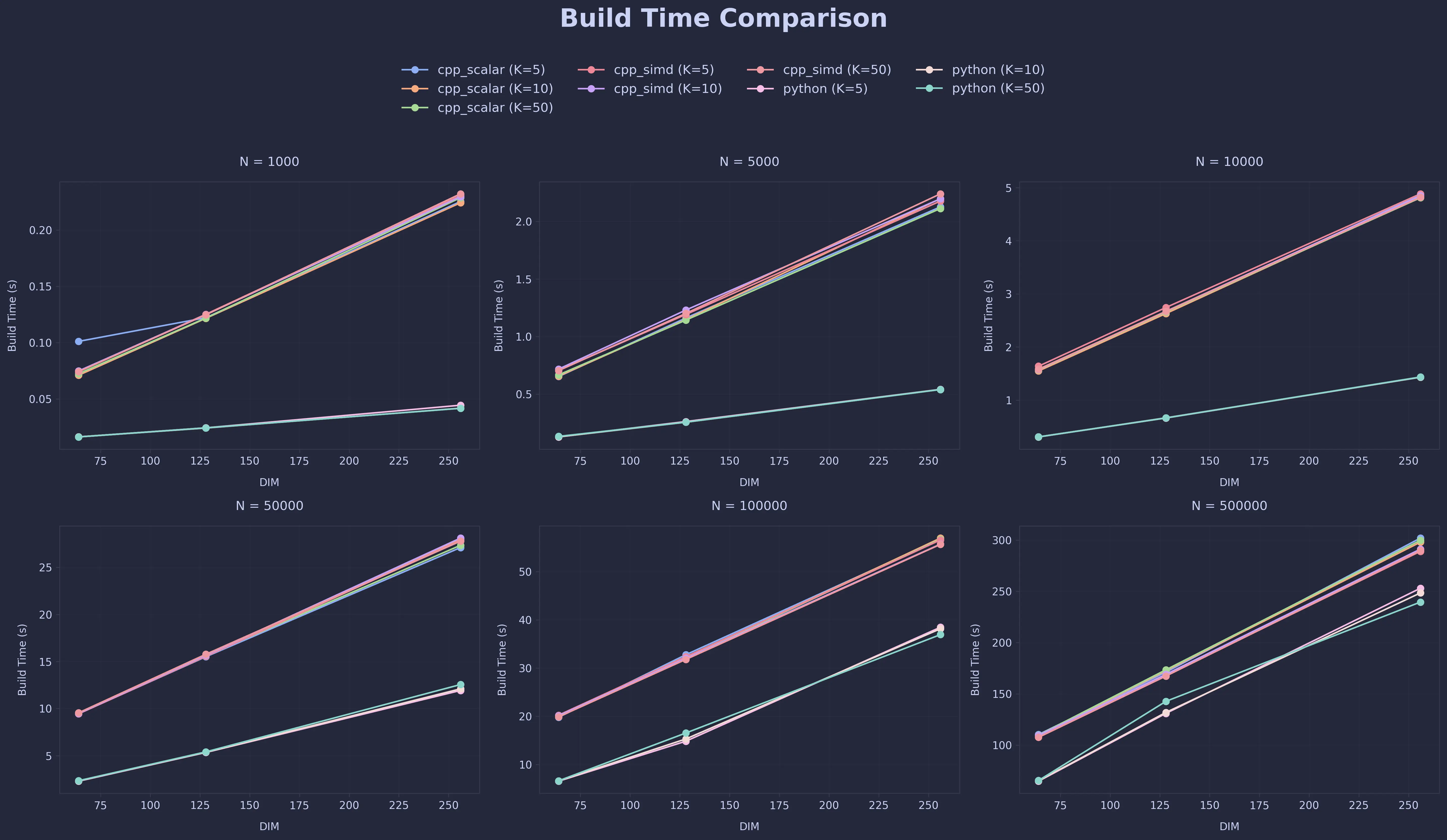
Plots For The Other Cases
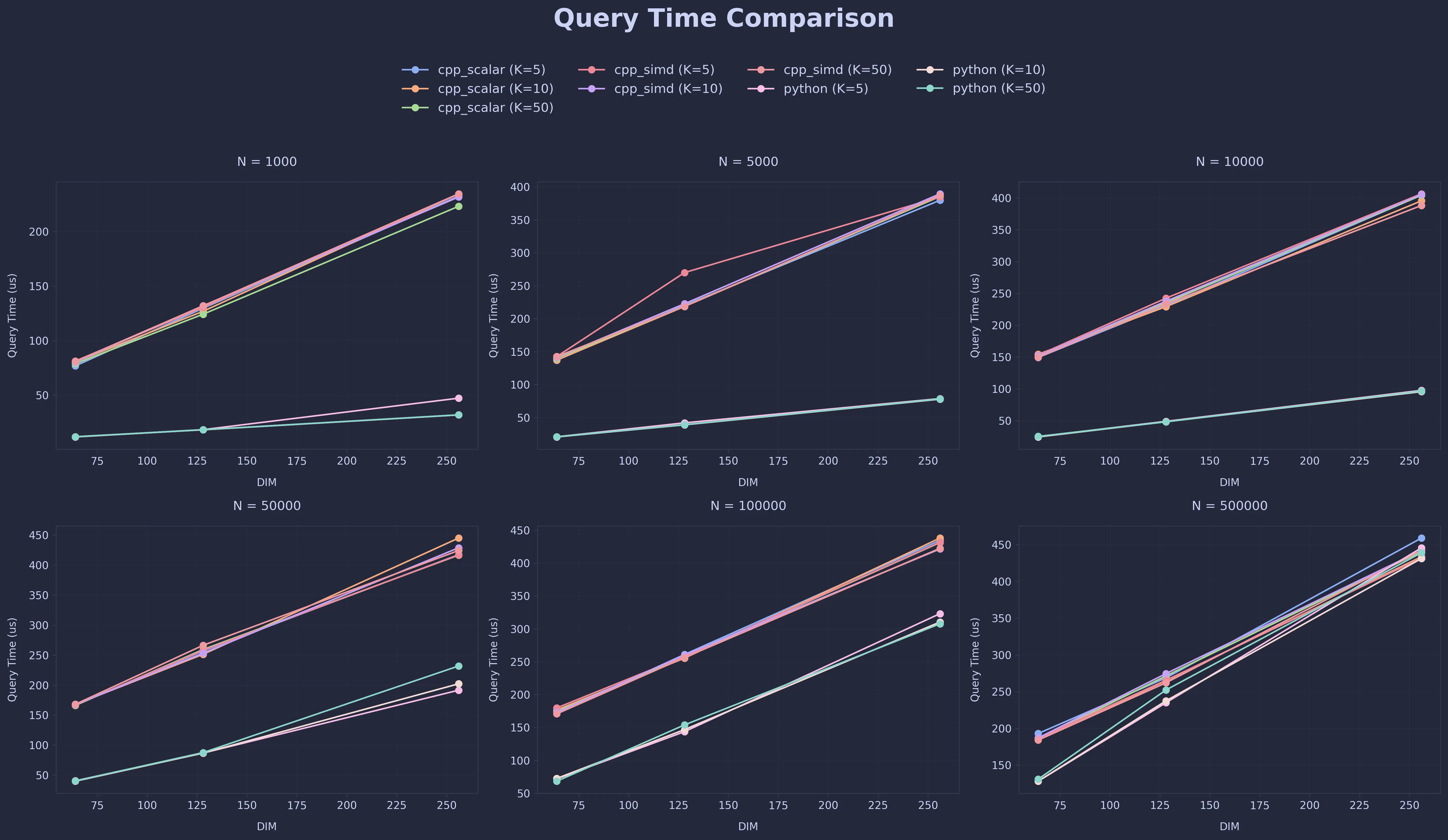
Once again, all these plots are available on my GitHub repo as proper PNGs
Build Time Comparison
Query Time Comparison
Conclusion
For small datasets, a well-implemented brute-force search can already be surprisingly competitive. But as datasets grow, approximate nearest neighbor methods like HNSW become far more efficient.In my experiments, moving from a naive implementation to a more optimized one improved build and query times by ~80–100×. Most of the gains came from fixing fundamentals :
- better memory layout
- fewer allocations
- improved cache locality
These changes alone reduced build time for a 100k dataset from ~15 minutes to under a minute.
One thing that surprised me was the results from SIMD acceleration. The gains were much smaller than I had expected, so clearly, the query pipeline was still largely dominated by graph traversal and memory access
Compared to hnswlib, my version is still slower on small datasets, but the gap shrinks as the dataset grows, which suggests the core structure is sound. But in my defence, this project wasn’t about beating existing libraries, it was about understanding how these ANN systems work under the hood.
Also ... C++ gives you a TON of control. As Bjarne Stroustrup (creator of C++) put it:
“C makes it easy to shoot yourself in the foot; C++ makes it harder, but when you do, it blows your whole leg off.”
After finishing this project, I'm pretty sure my brain got blown off too. Totally worth it though 😭😎
Comments