I Fixed a Neural Network That's Supposed to Print Its Own Weights

A Bit Of Context

In the previous blog post, we were able to kind of get a neural quine, but we faced a 0-quine issue, i.e., all the weights were zero, so the output was all 0s. Technically speaking, it's a valid solution but I don't want that. As mentioned in the previous post, this was researched around 8 years ago in this paper Neural Network Quine, 2018 and I dove straight into implementing it without reading it 😭.

Problems Faced

1. The zero-quine problem

   • If all weights are zero, the network trivially satisfies $F(0) = 0$.
   • Newton’s method or gradient descent will often converge to this trivial solution if the initialization isn’t perfect.

2. Jacobian scales poorly

   • For a network with $P$ parameters, the Jacobian $J$ is $P \times P$.
   • Constructing, storing, and solving linear systems with $J - I$ becomes expensive and numerically unstable for even modest networks.

3. Nonlinear interactions and ill-conditioning

   • Neural quines are highly coupled : changing one weight affects multiple outputs. So, Newton’s method oscillates or overcorrects

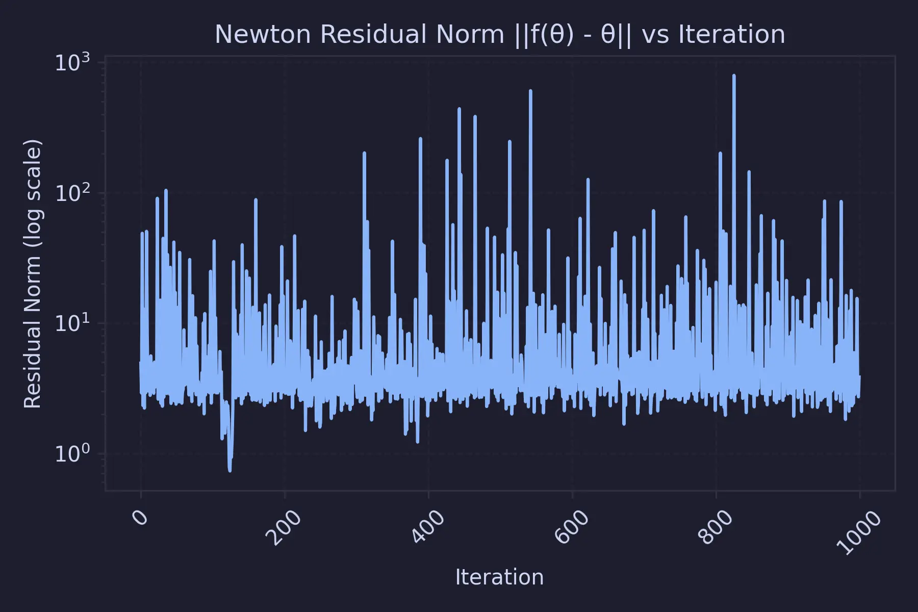
   • Newton’s method for solving the fixed-point equation

     $$ F(\theta) = \theta $$

     is locally stable only if

     $$ \min_i \left| \lambda_i\left(J_F(\theta^*)\right) - 1 \right| > 0. $$

     Instability occurs when any eigenvalue of $J_F$ satisfies this. That's why we see unstable losses using this method :

So, in this post, we will be going in a more "educated" direction to solve this puzzle.

What Does The Paper Say ?

Earlier, we were modeling the whole quine puzzle as a regression problem with multiple outputs ... this paper does something clever and interesting. The method described in this paper sort of makes the input "control" the output. The way it does that is by making the weights of the entire neural network queryable.

So, inp[i][j] = W_ij ... This is achieved by using a one-hot encoding to indicate which weight is currently being queried :

This seems like a neat idea, but the only thing that bothered me was : we must loop over all indices to reconstruct $\theta$.

Apart from that, the paper also evaluates various standard optimizers like RMSProp, Adam, etc., during the regeneration phase. (I'll also be migrating to that as things seem a bit more comfortable after seeing such common terms 😭)

What Did I Do ?

Instead of doing that, I store a fixed input_probe and condition the whole neural network on that probe. Formally, my model is defined as:

Where :

• $d = 8$ (input dimension)
• $P$ = total number of parameters
• $\theta \in \mathbb{R}^P$ is the flattened parameter vector

We choose a fixed probe vector :

And train the network so that :

The cool thing about this is that we need only a single forward pass to generate the entire parameter vector. Training the model solves the nonlinear fixed-point condition :

This means the parameters define a function that, when evaluated at a specific input $z$, outputs those same parameters. So now, the input does not need to be size $P$. The model learns this mapping :

Weirdly, this change has nothing to do with the model architecture at all, to be honest. model.py still remains the same :

 1class Quine(nn.Module):
 2    def __init__(self, alpha=0.25):
 3        super().__init__()
 4        self.alpha = alpha
 5
 6        self.l1 = nn.Linear(8, 20)
 7        self.l2 = nn.Linear(20, 20)
 8        self.l3 = nn.Linear(20, 20)
 9
10        self.P = sum(p.numel() for p in self.parameters())
11
12        # Fixed random projection
13        proj = torch.randn(20, self.P) / 20.0
14        self.register_buffer("proj", proj)
15
16        self.activation = nn.Tanh()
17
18    def forward(self, z):
19        x = self.activation(self.l1(z))
20        x = self.activation(self.l2(x))
21        x = self.activation(self.l3(x))
22        out = x @ self.proj
23        return self.alpha * out
24
25
26def flatten_params(model):
27    return torch.cat([p.view(-1) for p in model.parameters()])
28
29def set_params(model, theta_vec):
30    idx = 0
31    with torch.no_grad():
32        for p in model.parameters():
33            num = p.numel()
34            p.copy_(theta_vec[idx : idx + num].view_as(p))
35            idx += num

The only thing that has changed is the inputs. Earlier, in Part 1, I used fixed inputs because I thought the "ideal quine should ignore the inputs.". In this approach, we do something like this :

 1model = Quine(alpha=0.25).to(device)
 2theta = flatten_params(model).detach().clone().requires_grad_(True)
 3
 4# Fixed random seed / fixed z
 5input_probe = torch.randn(1, 8).to(device)
 6
 7optimizer = torch.optim.RMSprop([theta], lr=1e-3)
 8loss_list = []
 9
10num_steps = 200000
11
12for step in tqdm(range(num_steps), desc="Training Progress", unit="step"):
13    optimizer.zero_grad()
14
15    set_params(model, theta)
16
17    pred = model(input_probe).view(-1)
18    loss = torch.norm(pred - theta) ** 2
19
20    loss.backward()
21    optimizer.step()
22
23    loss_list.append(loss.item())
24
25    if step % 500 == 0:
26        tqdm.write(f"Step {step:04d} | Loss = {loss.item():.3e}")
27
28# Final pass
29set_params(model, theta.detach())

Hmmm, But How Does This Prevent 0-Quines ?

I had the same question. All we did was change the structure a bit but after the set_params method is called, if the weights ever became 0, there's no way to update them. Reason being, the gradients will also be 0 in the subsequent iterations as we literally just replace the weights.

To bypass this, I followed a clever trick from Evan Fletcher’s blog (should've read this before too 😭 ... it's pretty good):

We can forcibly avoid the zero quine by adding a parameter-free normalization layer after the trained dense layer. Both instance normalization and batch normalization (with all learned & running parameters disabled – no extra weights!) produce imperfect, but non-trivial, quines with relatively low error.

This works because, even though the weights can be zero, the gradients never are. Here's my proof attempt (kindly correct me if I'm mistaken anywhere) :

Coming back to code, adding this changes the model a bit : (we can use either InstaceNorm1d or BatchNorm1d here, I went with the former)

 1class Quine(nn.Module):
 2    def __init__(self, alpha=0.25):
 3        super().__init__()
 4        self.alpha = alpha
 5
 6        self.l1 = nn.Linear(8, 20)
 7        self.l2 = nn.Linear(20, 20)
 8        self.l3 = nn.Linear(20, 20)
 9
10        self.norm1 = nn.InstanceNorm1d(20, affine=False)
11        self.norm2 = nn.InstanceNorm1d(20, affine=False)
12        self.norm3 = nn.InstanceNorm1d(20, affine=False)
13
14        self.P = sum(p.numel() for p in self.parameters())
15
16        # Fixed random projection
17        proj = torch.randn(20, self.P) / 20.0
18        self.register_buffer("proj", proj)
19
20        self.activation = nn.Tanh()
21
22    def forward(self, z):
23        x = self.activation(self.l1(z))
24        x = self.norm1(x.unsqueeze(0)).squeeze(0)
25
26        x = self.activation(self.l2(x))
27        x = self.norm2(x.unsqueeze(0)).squeeze(0)
28
29        x = self.activation(self.l3(x))
30        x = self.norm3(x.unsqueeze(0)).squeeze(0)
31
32        out = x @ self.proj
33        return self.alpha * out

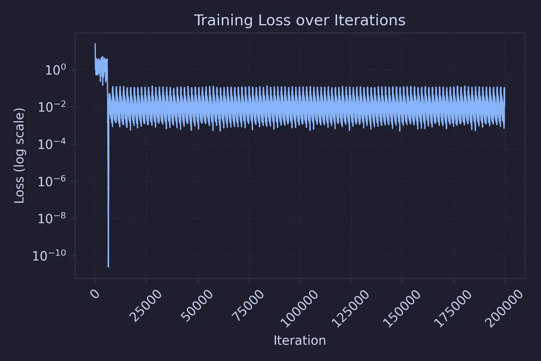
This is how the training loss graph looks like :

Model Results

This time, things look positive. After training the model with the following configurations :

1model = Quine(alpha=0.25)
2optimizer = torch.optim.RMSprop([theta], lr=1e-3)
3num_steps = 200000

These are the results :

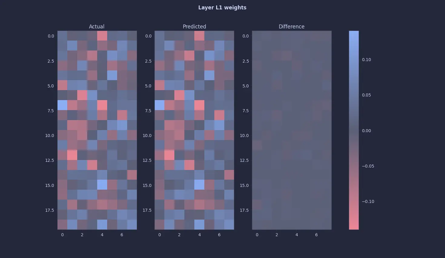
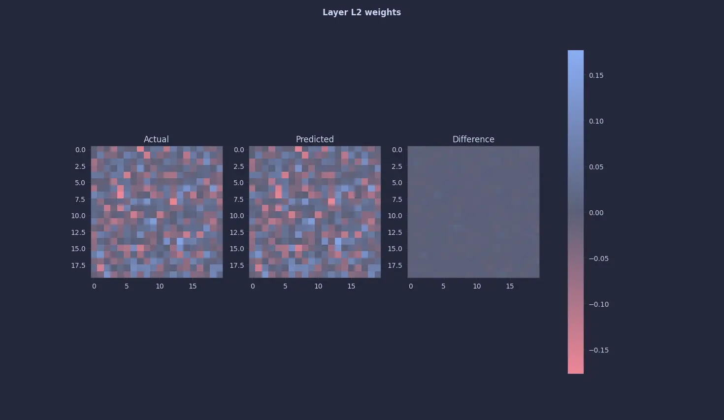
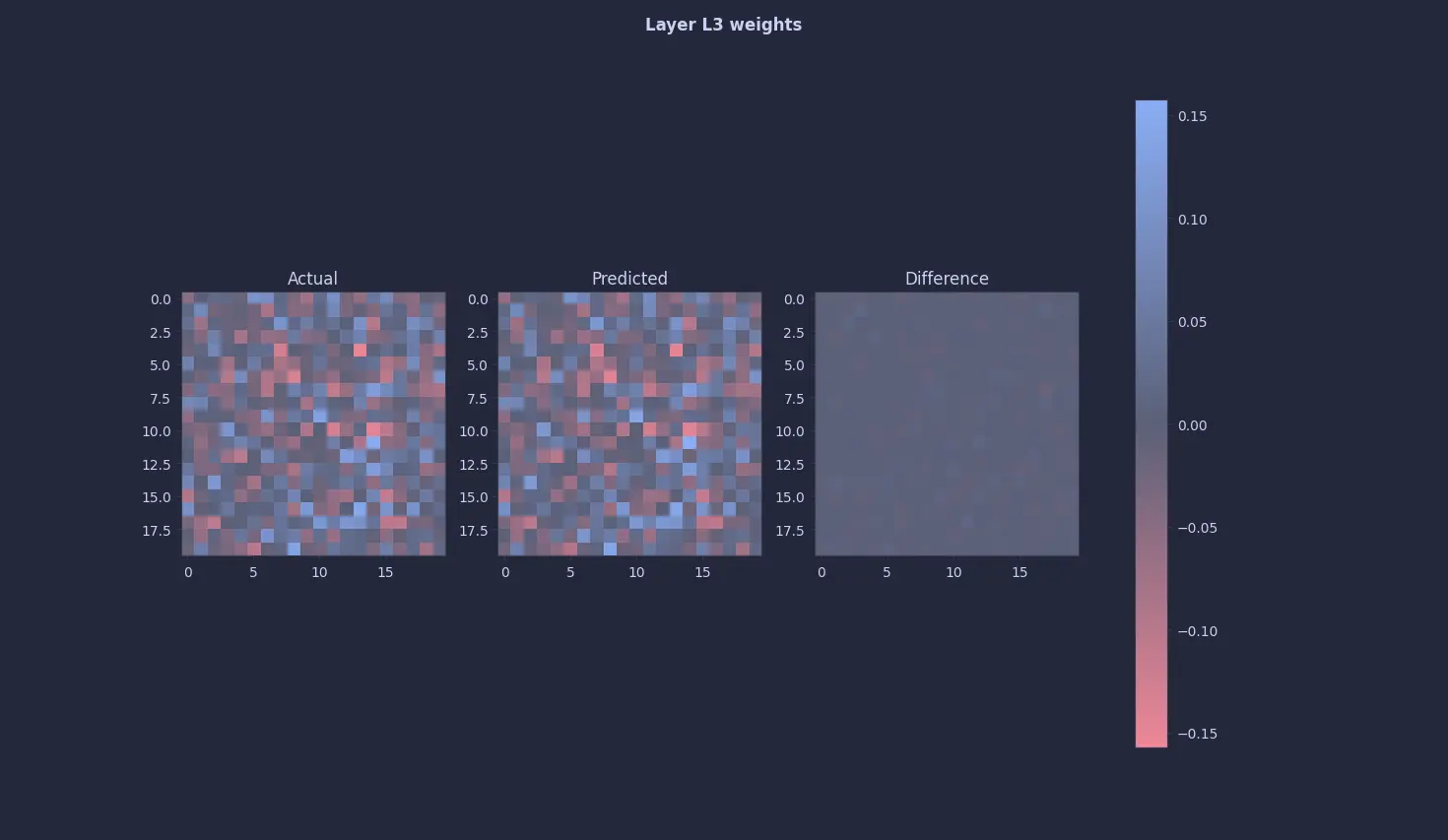
Finally 🥹🥹. A quine 🥹🥹

Conclusion

Although we were able to get a neural network to print its own weights, one might argue that this is technically not a true quine, as the differences between the weights are not exactly 0. And to those people I say "Please. Let me have this moment 😭".

In all seriousness though, they are right. It is almost impossible to get a perfect quine for many reasons. One that comes to mind is simply numerical precision on machines. But, we can get the delta to be as close to 0 as possible. Something in the range of (±10⁻¹⁵) seems decent to me.

Anyhow, for now, I'm happy with the results. But in a later post (in the distant future), we will explore whether this can be replicated in more complex models like CNNs, RNNs, LSTMs and Transformers