I Made A Neural Network That Prints Its Own Weights

How I Got The Idea

I saw this beautiful video by Dylan Beattie called Art of Code a few years ago, and I was fascinated by the idea of quines. Quine , as Wikipedia puts it, is basically a program (with no inputs) that prints its own source code. The video linked above goes a step further and introduces a polyquine (a program which outputs the source of a different program in another programming language) and finally enlightens us with the ever-amazing quine-relay (It’s a Ruby program that generates a Rust program that generates a Scala program that generates ... (through 128 languages in total) ... a REXX program that generates the original Ruby code again).

Now, I might like weird and esoteric stuff, but I’m not smart enough to code a quine-relay 🙏. But, I do like machine learning and I wanted to see if I could do something analogous to a quine but in ML sense.

Modelling The Problem

So, we want to have a neural network that outputs it’s own weights. Initially, I modeled the whole thing as a regression problem with multiple outputs. The idea was simple : treat the WHOLE neural network as a function $F_\theta(z)$ and try to make it output its own flattened parameters $\theta$ :

The loss could then be written as:

and in principle, I could train the network using gradient descent or even Newton’s method if I computed the full Jacobian:

If we introduce a scaling factor $\alpha$ for the quine (to control the magnitude of self-replication), the loss becomes:

The Jacobian now includes the scaling :

And the Newton-style update is updated accordingly:

The loss required a Jacobian because $F_\theta(z)$ depends on $\theta$, so we can’t just update the weights as-is; that would be like laying railway tracks while the train is already running.

Anyhow, this method allows you to control the "strength" of the quine with $\alpha$ while still using the Jacobian for Newton updates. This approach is mathematically neat, as it provides an exact fixed-point iteration — but in practice, there were several problems that I encountered later 🫠 (In Part 2, we solve these)

For now, I chose a simple feedforward network (I think it should work for other models as well but I’m not sure so don’t quote me on this 😅) :

 1class Quine(nn.Module):
 2    def __init__(self, alpha=0.25):
 3        super().__init__()
 4        self.alpha = alpha
 5
 6        self.l1 = nn.Linear(8, 20)
 7        self.l2 = nn.Linear(20, 20)
 8        self.l3 = nn.Linear(20, 20)
 9
10        self.P = sum(p.numel() for p in self.parameters())
11
12        proj = torch.randn(20, self.P) / 20.0
13        self.register_buffer("proj", proj)
14
15        self.activation = nn.Tanh()
16
17    def forward(self, z):
18        x = self.activation(self.l1(z))
19        x = self.activation(self.l2(x))
20        x = self.activation(self.l3(x))
21        out = x @ self.proj
22        return self.alpha * out

Here, we assign the output layer’s dimension based on the total parameters in the network (self.P). And note that the self.proj is NOT tracked by PyTorch's autograd engine ... and we want it that way.

self.proj is acting like a random fixed projection. Its job is just to map the 20-dimensional hidden representation into the huge output vector of length self.P. If we made it learnable, PyTorch would compute gradients for it and update it during training. That would defeat the purpose. We want the network to learn to output its own parameters, not to learn the projection itself. Hence, they are implemented using the register_buffer method

Training The Model

A question one might have is “What about the inputs ? How will the output change depending upon the input ?”. This is where things got a bit tricky for me as well. I had thought the “ideal quine” should technically ignore the inputs altogether. And it makes sense right ? Have the first layer’s weights as all 0s so that sort of takes away the dependency of output from the input.

That seems fine but an even trickier thing is … what exactly are the inputs here ? and, since it’s an ML problem, we should have some dataset, right ? What even is the dataset here ? Well, according to a quine, a program takes no input so going by that definition, in this case, we can use any fixed input as it “ideally should not matter at all”. Regarding the dataset, there is no dataset. This is more of a semi-supervised learning problem so in the loss function, the target value is LITERALLY the model’s current weights.

Dealing with all the weights as a matrix becomes a bit messy so I chose a linear approach with these utils :

 1def flatten_params(model):
 2    return torch.cat([p.view(-1) for p in model.parameters()])
 3
 4
 5def set_params(model, theta_vec):
 6    idx = 0
 7    with torch.no_grad():
 8        for p in model.parameters():
 9            num = p.numel()
10            p.copy_(theta_vec[idx : idx + num].view_as(p))
11            idx += num

Alright, all that is good. What about the weight updates ?! Since we have no backprop, how exactly are the weights updated ? I solve this by just replacing the weights by the learned weigths (this, as I found out later in that paper, is called “regeneration” 😭). So, the training loop looks a bit different from the usual ones :

 1
 2model = Quine(alpha=0.25).to(device)
 3
 4from torch.func import functional_call
 5
 6# We will use this while computing the Jacobian
 7def F(theta_vec):
 8    param_dict = {}
 9    idx = 0
10    for name, p in model.named_parameters():
11        num = p.numel()
12        param_dict[name] = theta_vec[idx:idx+num].view_as(p)
13        idx += num
14
15    
16    # UPDATE : This was wrong. This messes up the backprop graph as calling 
17    # model(...) will ignores theta_vec ... so F won't depend on theta_vec 
18    # and the Jacobian becomes zero
19    # return model(fixed_input).view(-1)
20    
21    return functional_call(model, param_dict, (fixed_input,)).view(-1)
22
23# This is just the loss function : F(theta) - theta
24def g(theta_vec):
25    return F(theta_vec) - theta_vec
26
27theta = flatten_params(model).detach().clone().requires_grad_(True)
28
29# This takes more than an hour on Macbook M4 and it oscillates. So, sticking 
30# with a lower number
31# num_steps = 200000
32num_steps = 1000
33tol = 1e-16
34
35
36for it in tqdm(range(num_steps), desc="Newton Progress"):
37
38	# We don't update the weights ... we just replace them
39    with torch.no_grad():
40        g_val = g(theta).detach()
41
42		# Sort of like the loss
43        norm = torch.norm(g_val).item()
44        residual_norms.append(norm)
45
46    tqdm.write(f"Step {it:02d} | ||g|| = {norm:.6e}")
47
48    if norm < tol:
49        print("Converged")
50        break
51
52    # Compute Jacobian and solve linear update
53    J = torch.autograd.functional.jacobian(F, theta)
54    A = J - torch.eye(P, dtype=J.dtype)
55
56    delta = torch.linalg.solve(A, g_val)
57    theta = (theta - delta).detach().requires_grad_(True)

Once training is done, we fix the model weights :

1set_params(model, theta.detach())
2final_out = model(fixed_input).view(-1).detach()
3final_theta = flatten_params(model).detach()
4diff = final_out - final_theta
5
6print("\nFinal ||difference|| : ", torch.norm(diff).item())

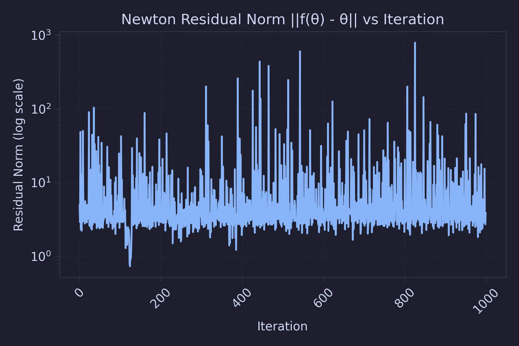
Training loss graph :

Model Results

The thing that I feared unfortunately occurred. Even by looking at the training loss graph, it's clear that the loss is oscillating. And it was around this time I learned something about Spectral Radius. The Newton’s method for solving the fixed-point equation :

is locally stable only if

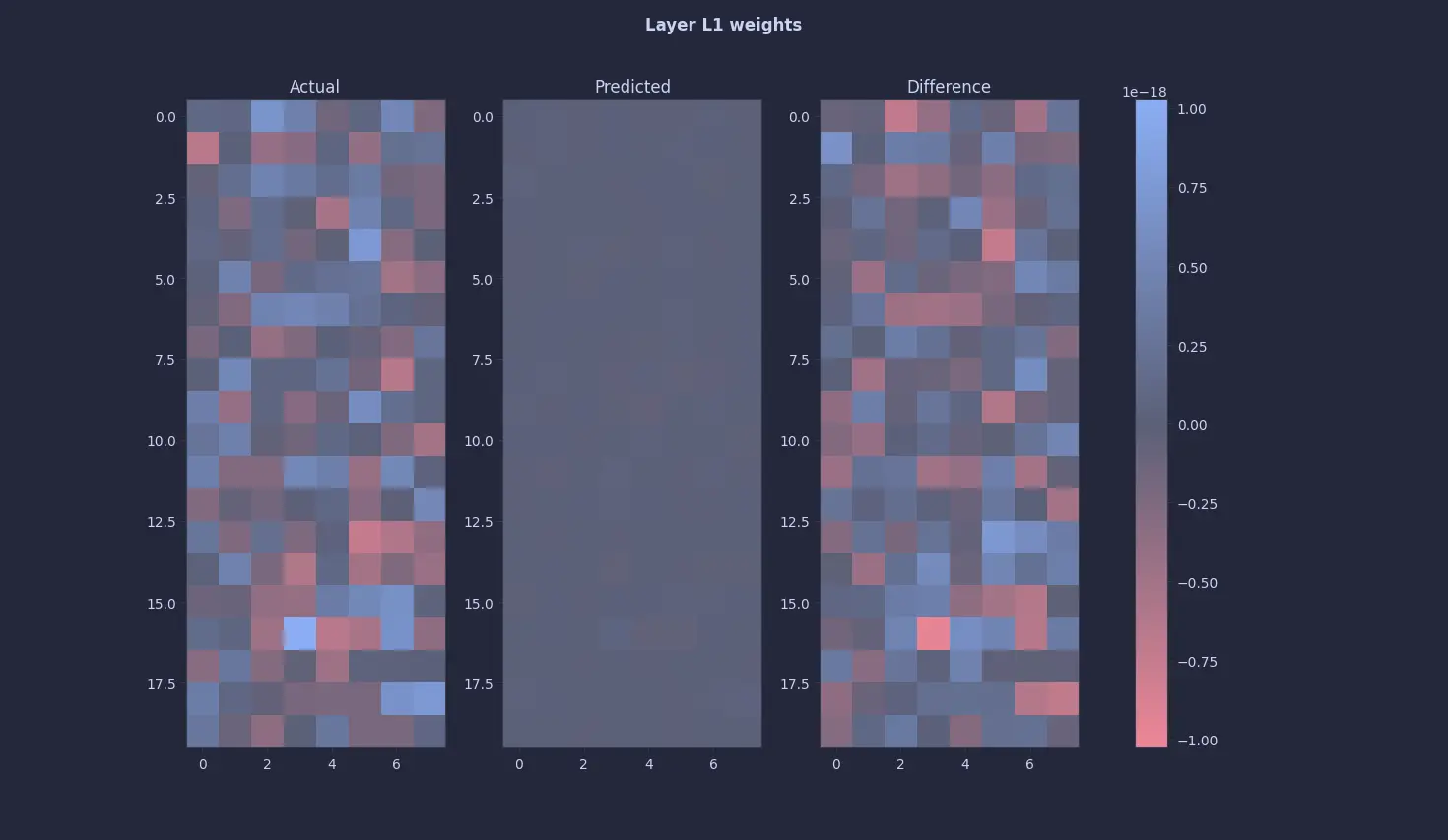
Instability occurs when any eigenvalue of $J_F$ satisfies. That's why we see unstable losses using this method. But, the first layer’s results looked promising as it was almost all 0 or close to 0 (~ 10^-18). So, my initial thought process was right - the model ignores the input altogether.

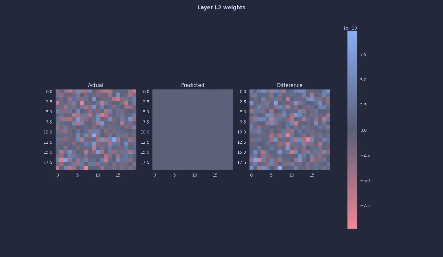
This seemed too easy so just to be sure, I looked at the 2nd and the 3rd layers … and they were all 0s (or close to it) too 😭 :

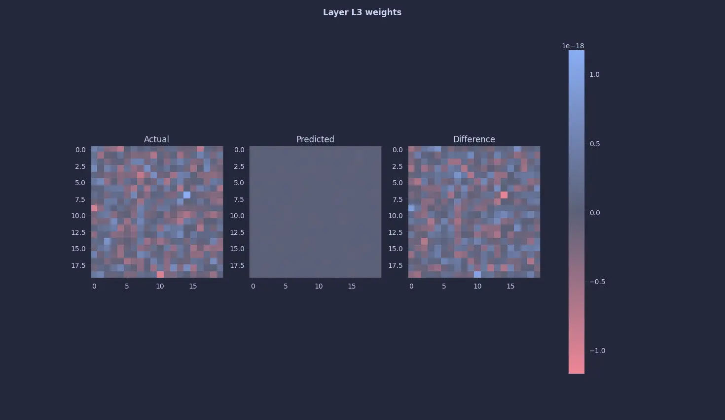
The annoying thing is, this was not a bug per se. To the above equation, all zeros is a perfectly valid fixed point or a solution. I knew a 0-quine would occur, so I tried desperately tweaking every knob and even the entire architecture, but it’s just a valid solution … all this to figure out that 0 = 0 🫠

So, Did We Get A “Neural Quine” ?

Well, yes. It’s technically right but that’s cheating if you ask me. It reminds me of this scene from Silicon Valley :

So, there were few extra steps I took to fix this and finally read the paper (🫠) to know how they did it. In part 2, we'll show a proper quine (which is not a 0-quine) that outputs it's own weights