I Tried Using DL To Optimize Python’s Garbage Collection (1/2)
How I Got This Idea
One of my friends was building an RL based system to train bipedal walker to … well walk. Ideally, one would use libraries like Gym, NEAT, etc but he was stubborn and wanted to build everything from scratch. Anyhow, during that process, he used things like the foot’s angular momentum, hand’s velocity, torso’s energy and whatnot to feed into a neural network to see how it performs. That’s when it struck me : why not use a similar approach to something low level ? Now, I haven’t yet gone through CPython’s internal implementation of these things so for the time being I’m gonna stick to the Python world. This allows me to treat GC as something I can influence externally rather than modify internally.
Repo for this whole thing along with detailed explanations, architecture diagrams, usage, etc can be found here
Why ? Isn’t GC Related Issues Prevalent In Java ?
True. GC pauses can cause memory spikes which can result in OOM errors and it can also have other performance related issues. In fact, Java was going to be my language of choice for this specific experiment because a LOT of things can be tuned in Java’s GC … heck even the GC itself can be switched with multiple implementations.
And even from a machine learning standpoint, that’s nice right ? More knobs mean more dimensions for the model to explore and optimize … so why not use Java ? Well, the reason is simple. I’m not that proficient in Java 😅
I could use ChatGPT and get a server running and somehow figure out a way to invoke the garbage collector .. but I’ll be using PyTorch for my models and to get that up and running on a Java process seems like a chore. So, for this post, I decided to use Python end-to-end.
Python primarily manages memory using reference counting. This means that when an object’s reference count drops to zero, its memory is freed immediately, without involving the garbage collector at all.
As a result, you can’t trigger meaningful GC activity just by creating and deleting a lot of short-lived objects. To actually exercise Python’s garbage collector, you need to create reference cycles (for example, objects that reference each other), because these won’t be reclaimed by reference counting alone and require an explicit GC pass to clean up.
Alright Okay 😓 What Next ..
Input / Output
Now, for any ML model, the first question is : what are the inputs and outputs ?
Well, output is straightforward as it’s a binary classification problem. If our model predicts a value greater than some threshold, trigger the gc call using gc.collect().
The inputs are ... noisier to say the least. Since I’m not directly tapping into Python’s internal GC state, I use process-level metrics :
Choosing system metrics isn’t perfectly accurate because the “system” is running other processes as well. For example, 50% RAM usage doesn’t necessarily mean your application alone is using 50%.
To reduce this noise, I rely on process-level metrics instead of global system metrics.
 1
 2@dataclass
 3class ProfileMetrics:
 4    time : float = 0.0
 5    cpu : float = 0.0
 6    mem : float = 0.0
 7    disk_read : float = 0.0
 8    disk_write : float = 0.0
 9    net_sent : float = 0.0
10    net_recv : float = 0.0
11    rps : float = 0.0
12    p95 : float = 0.0
13    p99 : float = 0.0
14    gc_triggered : bool = False
The output is a single floating-point value between 0 and 1, which represents the model’s confidence that a garbage collection cycle should be triggered :
 1
 2mem_pressure = df["mem"].values / 100.0
 3cpu_factor = df["cpu"].values / 100.0
 4gc_recent = df["gc_triggered"].astype(float).values
 5
 6# Our Output
 7self.targets = np.clip(
 8    0.4 * mem_pressure + 0.3 * cpu_factor + 0.3 * (1 - gc_recent * 0.5),
 9    0.0,
10    1.0,
11).astype(np.float32)
In this implementation, I construct this target using a simple heuristic rather than directly tuning Python’s internal GC parameters. While it is possible to influence GC behavior by adjusting gc.set_threshold(), I deliberately avoid doing so here to keep the experiment simple
Model
Carrying the light hearted spirit of an “MVP”, I chose a dead simple LSTM based model. Since timestamps are involved and the data is sequential, LSTMs are a natural baseline for time-series behavior modeling :
 1class LSTMNetwork(nn.Module):
 2    def __init__(
 3        self,
 4        input_size: int = 10,
 5        hidden_size: int = 64,
 6        num_layers: int = 2,
 7        dropout: float = 0.2,
 8    ):
 9        super().__init__()
10
11        self.input_size = input_size
12        self.hidden_size = hidden_size
13        self.num_layers = num_layers
14
15        self.lstm = nn.LSTM(
16            input_size=input_size,
17            hidden_size=hidden_size,
18            num_layers=num_layers,
19            batch_first=True,
20            dropout=dropout if num_layers > 1 else 0,
21        )
22
23        self.fc = nn.Linear(hidden_size, 1)
24        self.sigmoid = nn.Sigmoid()
25
26    def forward(self, x: torch.Tensor) -> torch.Tensor:
27        lstm_out, _ = self.lstm(x)
28        last_output = lstm_out[:, -1, :]
29        out = self.fc(last_output)
30        out = self.sigmoid(out)
31        return out
Optimizers and Training
There are two main approaches here :
- Offline training : Profile an application under load, collect data, train a model, and then deploy the trained model alongside the application.
- Online training : Continuously update the model as new data comes in, with no fixed dataset.
I chose the offline approach. I wanted to see how a model trained specifically on a given application’s behavior would perform when reintroduced into that same environment.
For optimization, I used Adam with a learning rate of 1e-3 to keep things simple and stable.
Environment and Training
For the environment, I use a FastAPI based web server with the following endpoints to simulate the respective load-type : (these do things like calculate a bunch of prime numbers, open / read / close files, etc.)
1@app.get("/cpu-heavy")
2@app.get("/memory-heavy")
3@app.get("/network-heavy")
4@app.get("/io-heavy")
In addition to that, it also contains relevant code for running the profiler in the background and exposes an API to get the process’s metrics :
1@app.get("/metrics")
2async def get_metrics():
3    metrics = profiler.get_metrics()
4    data = metrics.to_dict()
5    # .. other processing ..
6    return data
The full code for these can be obtained here. For testing the server under low and high load, I’m using Locust. While training the ML model, I run the FastAPI server without NeuroGC (this is what I call it 🤓) .. load test it against Locust and profile relevant metrics from the server. Once that is done, train the model based on those metrics using a straight-forward torch training loop. After training is done, I save the model as a .pth file (for loading the model later)
Testing The Model
This involves a few things.
First, I create another
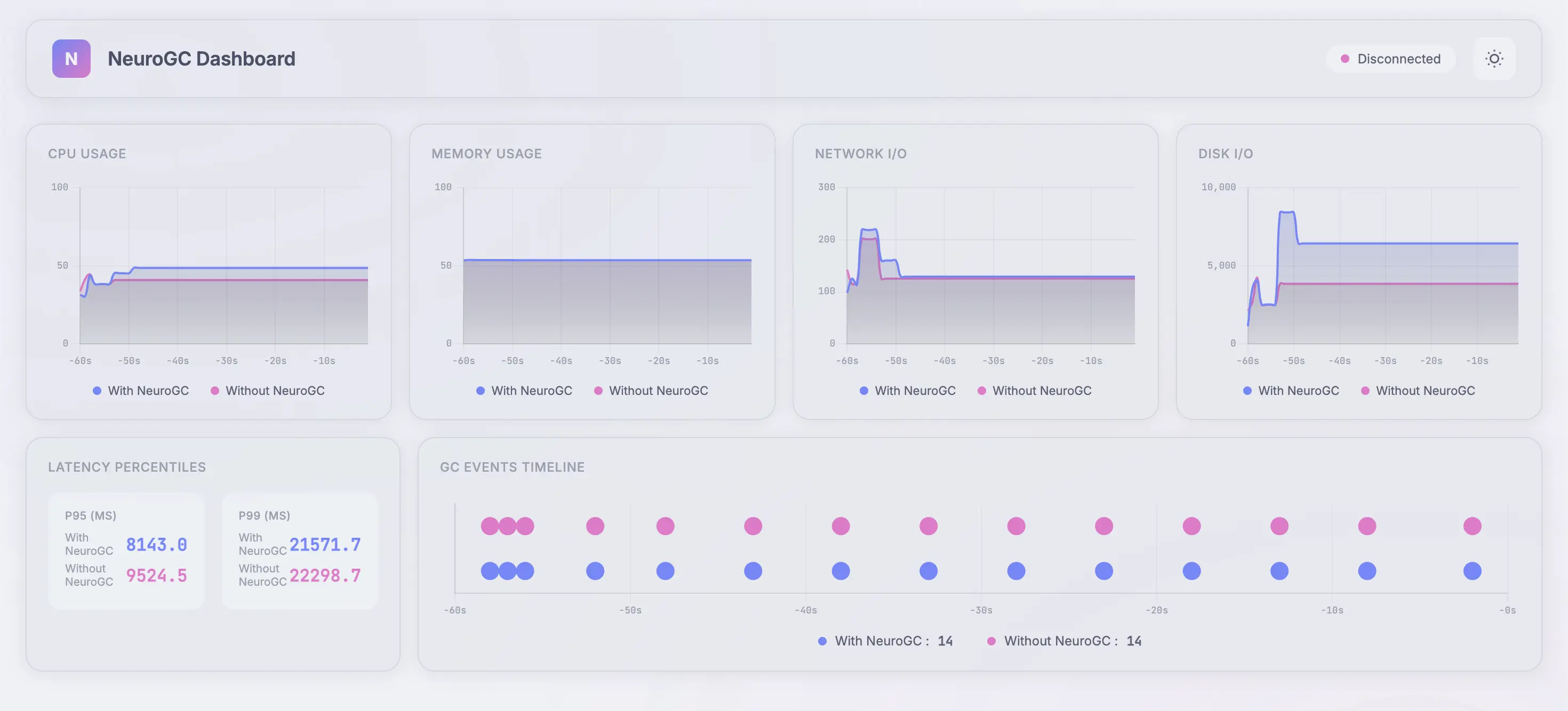
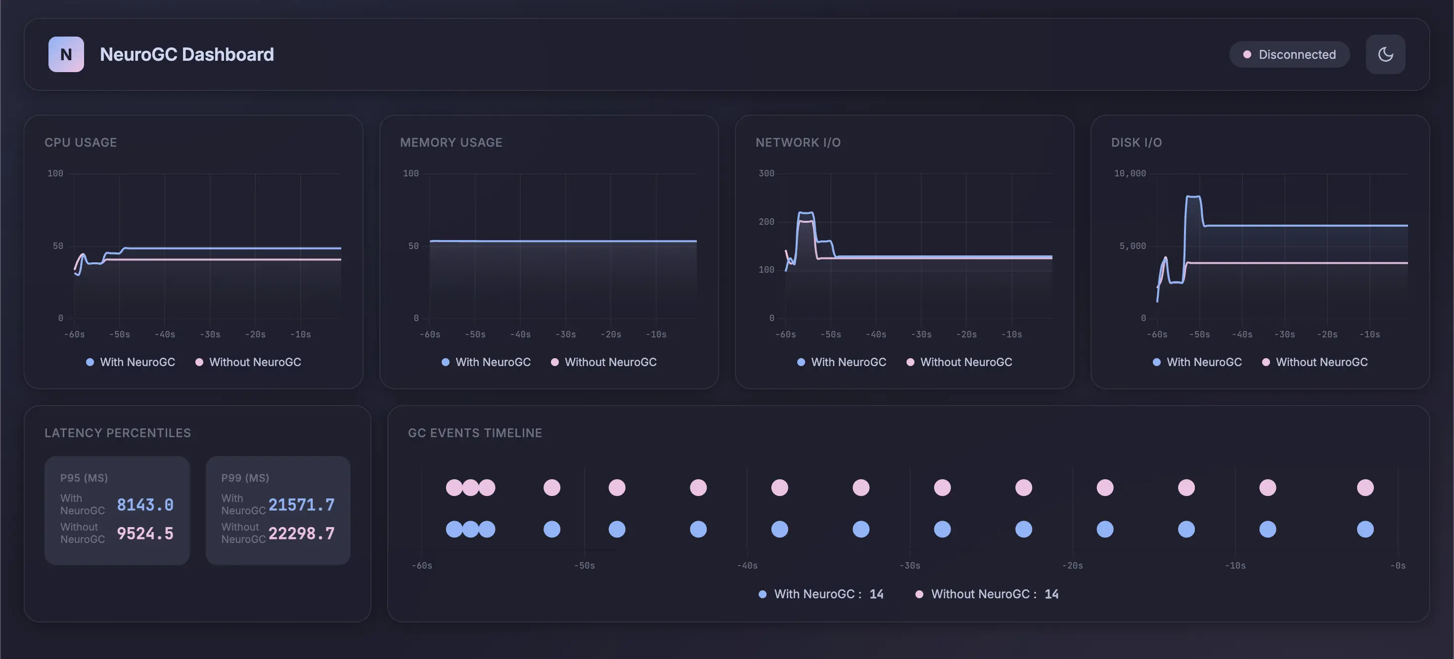
FastAPIbased web server (similar to the one mentioned above), but when it starts, I load the model and runNeuroGCin the background usingasyncio.create_task()method. This triggers (or does not trigger) GC based on the model’s predictionSecond, we need a way to see the metrics update in realtime. There are 2 types of metrics that I’m looking for. One is process-level metric like CPU, RAM, etc and the other is server performance metrics like p95, p99, etc. We already get the process metrics via the
/metricsendpoint. To get the other ones, we can useLocustas that is already making a ton of requests. We need to club these 2 together so that we can show all these in the UI. The glue code for that is a simple class that runs in the background of the Locust’s process :
 1class ProfileCollector:
 2    def __init__(
 3        self,
 4        profile_interval: float = 1.0,
 5        metrics_server_url: str = "http://localhost:8003",
 6    ):
 7        self.profile_interval = profile_interval
 8        self.metrics_server_url = metrics_server_url
 9
10        ...
11
12    ...
13
14    def _fetch_server_metrics(self) -> None:
15        try:
16            with httpx.Client(timeout=2.0) as client:
17                try:
18                    resp = client.get(f"{self.server_with_gc_url}/metrics")
19                    if resp.status_code == 200:
20                        self._server_metrics_with_gc = resp.json()
21                except Exception:
22                    pass
23
24                try:
25                    resp = client.get(f"{self.server_without_gc_url}/metrics")
26                    if resp.status_code == 200:
27                        self._server_metrics_without_gc = resp.json()
28                except Exception:
29                    pass
30        except Exception:
31            pass
32
33    def _run_loop(self) -> None:
34        while self._running:
35            try:
36                # Fetch actual metrics from each server
37                self._fetch_server_metrics()
38
39                metrics_with_gc = self._get_metrics_for_server("with_gc")
40                metrics_without_gc = self._get_metrics_for_server("without_gc")
41
42                # Send the metrics to metrics_server
43                try:
44                    with httpx.Client(timeout=5.0) as client:
45                        client.post(
46                            f"{self.metrics_server_url}/api/metrics",
47                            json=metrics_with_gc,
48                        )
49                        client.post(
50                            f"{self.metrics_server_url}/api/metrics",
51                            json=metrics_without_gc,
52                        )
53                except Exception:
54                    pass
55
56            except Exception as e:
57                print(f"[ProfileCollector] Error: {e}")
58
59            time.sleep(self.profile_interval)
60
61    def start(self) -> None:
62        self._running = True
63
64        if self.profiler:
65            self.profiler.start()
66
67        self._thread = threading.Thread(
68            target=self._run_loop,
69            daemon=True,
70        )
71        self._thread.start()
72
73        print(
74            f"[ProfileCollector] Started. Posting to {self.metrics_server_url}"
75        )
I use the @events.init.add_listener method and start the ProfileCollector on on_locust_init hook.
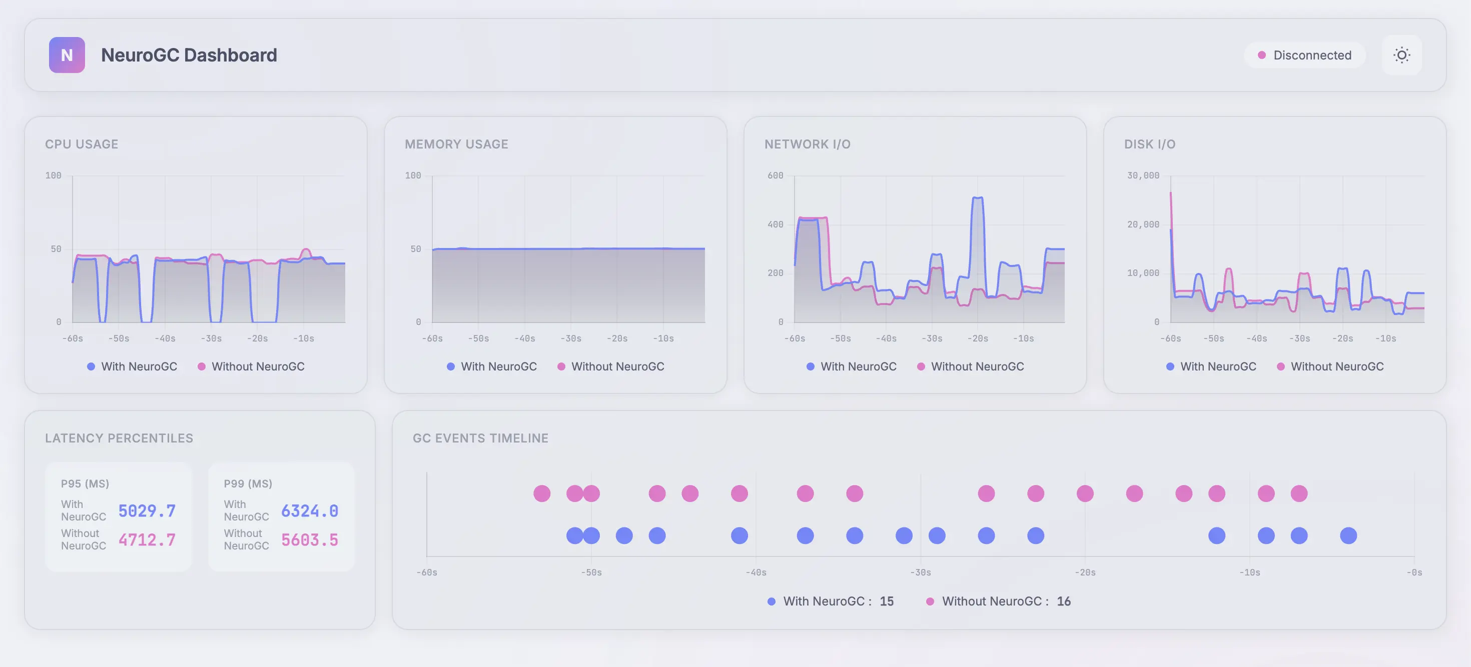
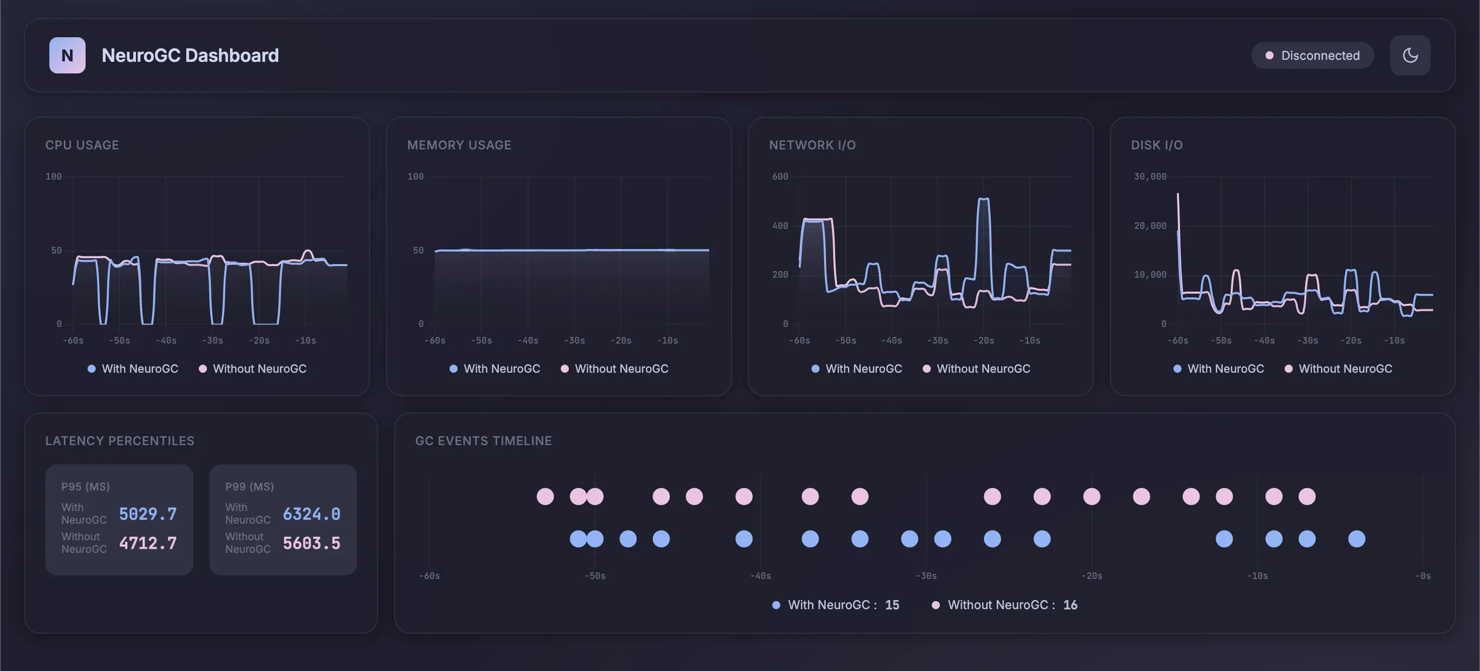
- Third, for seeing the metrics update in realtime, I didn’t want to involve a huge library like react for this project so I built a simple UI using
HTML,WebsocketsandCharts.js. The backend for this is yet another webserver called themetrics_server. It :- Serves the UI
- Gets the metrics from
Locustserver via the/api/metricsendpoint - Streams the latest metrics to the UI using a
Websocketconnection
… Too many servers, I know. I apologize 😭
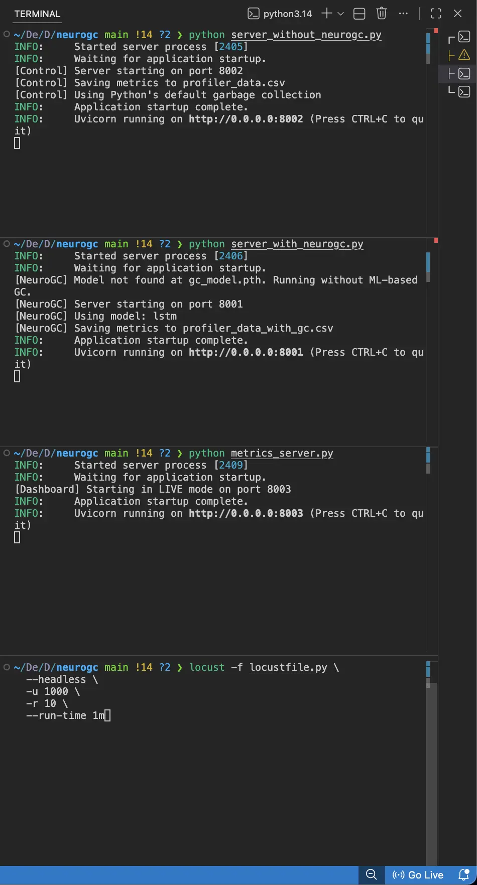
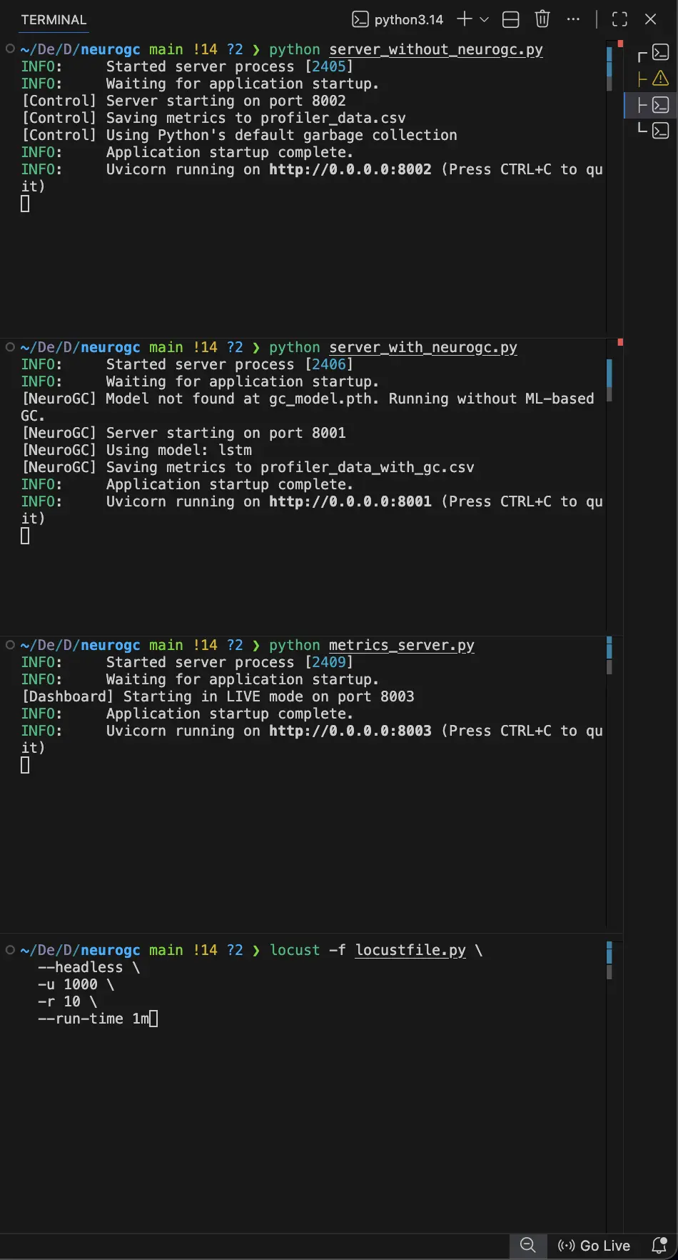
Anyhow, with that setup, we first start the servers with and without NeuroGC on 2 different terminals, then we start the metrics_server on another terminal and finally, start the Locust server on yet another terminal. The UI for the real-time dashboard can be viewed on localhost:8003
This might seem like a chore to do every time (if you are running this locally) …. I would suggest taking a look at tmux … maybe that will ease the process
Benchmarks
System Information
| Property | Value |
|---|---|
| Operating System | macOS 14.6 |
| Architecture | arm64 |
| CPU | arm |
| CPU Cores | 8 (logical: 8) |
| Memory | 24.0 GB |
| Disk | 460.4 GB |
| Python Version | 3.14.0 |
Light load
- Training Load :
locust -f locustfile.py --headless -u 100 -r 10 --run-time 1m - Evaluation Load :
locust -f locustfile.py --headless -u 100 -r 10 --run-time 1m
Full data :
| Metric | Without NeuroGC | With NeuroGC | Improvement |
|---|---|---|---|
| Avg CPU (%) | 38.0 | 29.0 | 🟢 +23.7% |
| Avg Memory (%) | 50.1 | 50.1 | 0.0% |
| Avg Disk Read | 14410.73 | 20069.47 | 🔴 -39.3% |
| Avg Disk Write | 9903865.30 | 6187022.12 | 🟢 +37.5% |
| Avg Net Sent | 81743.25 | 87163.18 | 🔴 -6.6% |
| Avg Net Recv | 102192.21 | 99026.00 | 🟢 +3.1% |
| P95 Latency (ms) | 3538.8 | 3609.9 | 🔴 -2.0% |
| P99 Latency (ms) | 4530.3 | 4769.2 | 🔴 -5.3% |
| Avg RPS | 31.2 | 30.7 | 🔴 -1.7% |
| GC Events | 19 | 17 | 🔴 -10.5% |
High Load
- Training Load :
locust -f locustfile.py --headless -u 500 -r 10 --run-time 1m - Evaluation Load :
locust -f locustfile.py --headless -u 500 -r 10 --run-time 1m
Full data :
| Metric | Without NeuroGC | With NeuroGC | Improvement |
|---|---|---|---|
| Avg CPU (%) | 40.2 | 43.2 | 🔴 -7.4% |
| Avg Memory (%) | 53.5 | 53.5 | 0.0% |
| Avg Disk Read | 10371.80 | 4011.52 | 🟢 +61.3% |
| Avg Disk Write | 6082227.94 | 5377198.66 | 🟢 +11.6% |
| Avg Net Sent | 68960.00 | 62821.57 | 🟢 +8.9% |
| Avg Net Recv | 78285.45 | 68550.20 | 🟢 +12.4% |
| P95 Latency (ms) | 4297.5 | 4424.6 | 🔴 -3.0% |
| P99 Latency (ms) | 9652.6 | 8373.4 | 🟢 +13.3% |
| Avg RPS | 29.5 | 28.6 | 🔴 -3.1% |
| GC Events | 15 | 15 | 0.0% |
Conclusion
With this LSTM-based approach, NeuroGC didn’t deliver a dramatic, across-the-board improvement and - that’s honestly not surprising.
What this experiment did show is that application behavior can be learned in a meaningful way using only high-level process metrics. Even with a relatively small dataset and a simple sequence model, the system was able to influence GC timing and, in some cases, reduce disk and network pressure under medium load.
That alone suggests there’s signal here … it’s just not being fully captured yet. In many ways, this LSTM model should be treated as a baseline rather than a final solution.
There are a few obvious directions for improvement :
- Larger datasets : Extending the load test duration from 1 minute to 10–30 minutes would significantly improve temporal coverage and reduce noise in the training data.
- Richer feature engineering : Adding derived signals (rates of change, rolling averages, memory allocation deltas, request burstiness) may give the model a clearer picture of why pressure is building.
- Stronger model architectures : Transformers, temporal convolutional networks, or even reinforcement learning could be better suited to learning long-term effects and delayed rewards in GC behavior.
- Online or hybrid training : Allowing the model to adapt as the application evolves might make it more robust in real-world deployments.
So while the LSTM didn’t didn’t significantly outperform Python's GC, it did something arguably more important :
It validated the idea that garbage collection can be treated as a learnable system rather than a fixed heuristic.
In Part 2 / 2, I’ll explore more expressive models, longer training runs, and whether this approach can move from “interesting experiment” to something that actually holds up under sustained production-level load. Wish me luck ! 😁🤞
Comments