I Tried Using DL To Optimize Python’s Garbage Collection (2/2)
Overview
In the previous blog post, we explored how we can use deep learning models to optimize Python's GC calls. In this post, we’ll look at how the model performs with :
- More training data
- More complex parameters
- More epochs
- Different model architectures
Thorough analysis with run-over-run metrics and Welch t-test for those can be found here.
System Information
| Property | Value |
|---|---|
| Operating System | macOS 14.6 |
| Architecture | arm64 |
| CPU | arm |
| CPU Cores | 8 (logical: 8) |
| Memory | 24.0 GB |
| Disk | 460.4 GB |
| Python Version | 3.14.0 |
Different Cases
Every model has the same training and evaluation load i.e. locust -f locustfile.py --headless -u 100 -r 10 --run-time 1m unless mentioned otherwise
Case 1 : Complex model
Model architecture is a normal LSTM but with more layers and increased sequence length :
1"lstm": {
2  "input_size": 10,
3  "hidden_size": 64,
4  "num_layers": 10,               // increased this from 2
5  "sequence_length": 100,         // increased this from 10
6  "epochs": 100,
7  "learning_rate": 0.001,
8  "batch_size": 32
9}
Realtime Monitor (pretty 😤) and Raw Results
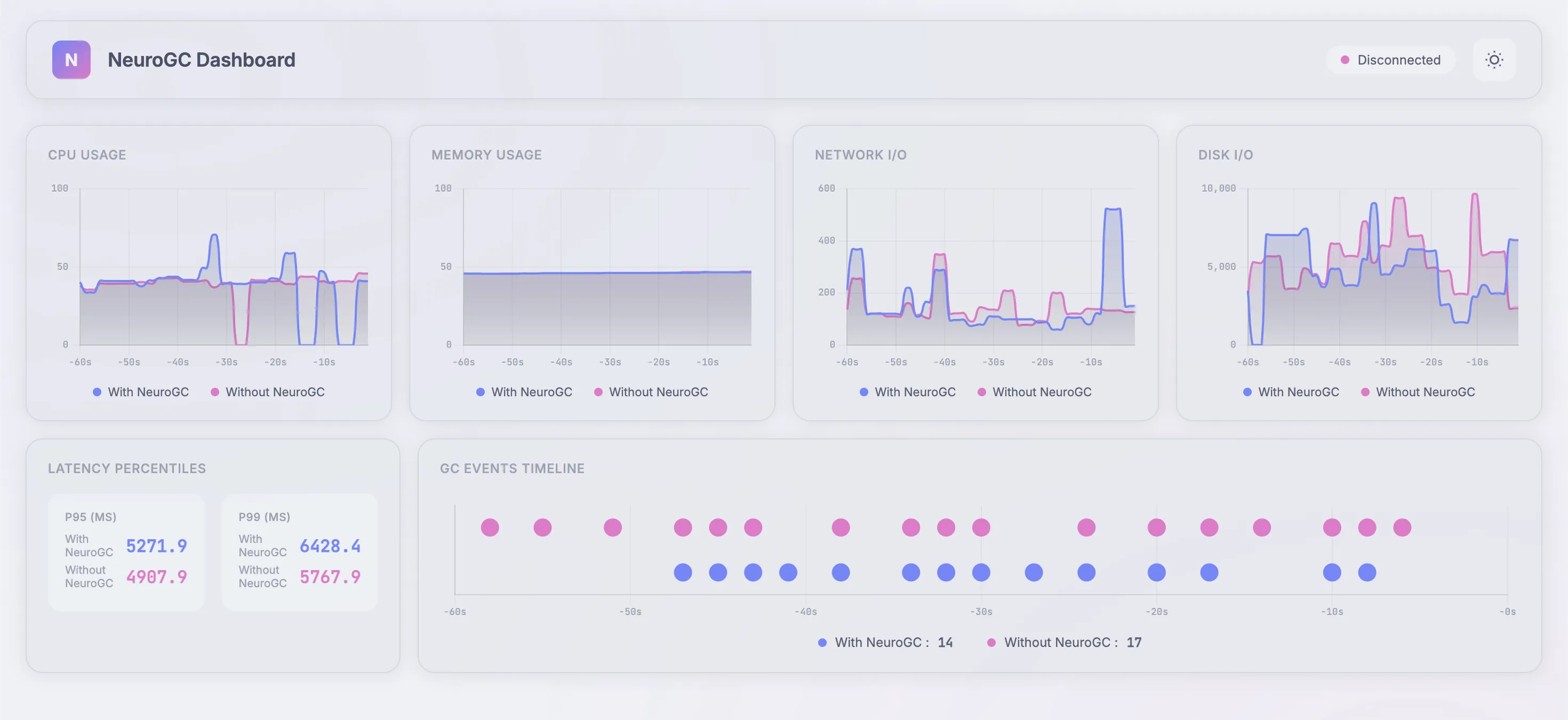
| Metric | Without NeuroGC | With NeuroGC | Improvement |
|---|---|---|---|
| Avg CPU (%) | 36.8 | 37.6 | 🔴 -2.1% |
| Avg Memory (%) | 46.1 | 46.1 | 🟢 +0.1% |
| Avg Disk Read | 8399.86 | 8133.23 | 🟢 +3.2% |
| Avg Disk Write | 5317931.93 | 4209032.94 | 🟢 +20.9% |
| Avg Net Sent | 67313.15 | 63477.44 | 🟢 +5.7% |
| Avg Net Recv | 74458.70 | 86484.33 | 🔴 -16.2% |
| P95 Latency (ms) | 3724.2 | 3751.8 | 🔴 -0.7% |
| P99 Latency (ms) | 4566.0 | 5080.4 | 🔴 -11.3% |
| Avg RPS | 29.4 | 28.2 | 🔴 -4.3% |
| GC Events | 18 | 15 | 🔴 -16.7% |
Case 2: Different model architecture
Here, we change the underlying ML model itself. Again, everything else follows the baseline config
Case 2a. Using normal feed-forward networks
We use the following config as baseline :
1"feedforward": {
2  "hidden_sizes": [64, 32, 16, 8],
3  "lookback": 20,
4  "epochs": 100,
5  "learning_rate": 0.001,
6  "batch_size": 32
7},
Realtime Monitor and Raw Results


| Metric | Without NeuroGC | With NeuroGC | Improvement |
|---|---|---|---|
| Avg CPU (%) | 39.8 | 43.0 | 🔴 -8.0% |
| Avg Memory (%) | 55.3 | 55.3 | 0.0% |
| Avg Disk Read | 7675.69 | 11055.08 | 🔴 -44.0% |
| Avg Disk Write | 5940870.38 | 8232453.21 | 🔴 -38.6% |
| Avg Net Sent | 93112.14 | 74657.59 | 🟢 +19.8% |
| Avg Net Recv | 95884.71 | 90835.58 | 🟢 +5.3% |
| P95 Latency (ms) | 3855.2 | 4139.6 | 🔴 -7.4% |
| P99 Latency (ms) | 5410.8 | 5231.7 | 🟢 +3.3% |
| Avg RPS | 29.8 | 29.3 | 🔴 -1.8% |
| GC Events | 14 | 18 | 🟢 +28.6% |
Case 2b. Using transformers
We use the following config as baseline :
1"transformer": {
2  "d_model": 64,
3  "nhead": 4,
4  "num_layers": 2,
5  "sequence_length": 10,
6  "epochs": 100,
7  "learning_rate": 0.001,
8  "batch_size": 32
9}
Realtime Monitor and Raw Results

| Metric | Without NeuroGC | With NeuroGC | Improvement |
|---|---|---|---|
| Avg CPU (%) | 37.5 | 33.7 | 🟢 +10.2% |
| Avg Memory (%) | 55.1 | 55.1 | 0.0% |
| Avg Disk Read | 2433.94 | 1638.77 | 🟢 +32.7% |
| Avg Disk Write | 6325593.39 | 5631381.21 | 🟢 +11.0% |
| Avg Net Sent | 116008.92 | 68573.32 | 🟢 +40.9% |
| Avg Net Recv | 98824.23 | 92021.42 | 🟢 +6.9% |
| P95 Latency (ms) | 3780.6 | 3718.8 | 🟢 +1.6% |
| P99 Latency (ms) | 4827.9 | 4913.1 | 🔴 -1.8% |
| Avg RPS | 29.8 | 30.6 | 🟢 +2.9% |
| GC Events | 18 | 17 | 🔴 -5.6% |
Case 2c. Using classical ML algorithms like Random Forest
We use the following config as baseline :
1"classical": {
2  "algorithm": "random_forest",
3  "n_estimators": 100,
4  "max_depth": null,
5  "lookback": 20
6}
Realtime Monitor and Raw Results


| Metric | Without NeuroGC | With NeuroGC | Improvement |
|---|---|---|---|
| Avg CPU (%) | 39.0 | 39.3 | 🔴 -0.8% |
| Avg Memory (%) | 54.4 | 54.5 | 0.0% |
| Avg Disk Read | 2786.16 | 591.43 | 🟢 +78.8% |
| Avg Disk Write | 6037546.50 | 5408297.63 | 🟢 +10.4% |
| Avg Net Sent | 90606.60 | 67460.24 | 🟢 +25.5% |
| Avg Net Recv | 97007.71 | 74088.75 | 🟢 +23.6% |
| P95 Latency (ms) | 3488.8 | 3450.9 | 🟢 +1.1% |
| P99 Latency (ms) | 4587.6 | 4786.3 | 🔴 -4.3% |
| Avg RPS | 30.4 | 29.9 | 🔴 -1.6% |
| GC Events | 16 | 19 | 🟢 +18.8% |
Case 3: With more training data
Training load is now for 5 minutes. Evaluation load remains the same :
1# Training load (increased to 5 mins)
2locust -f locustfile.py --headless -u 100 -r 10 --run-time 5m
3
4# Evaluation load (same as before)
5locust -f locustfile.py --headless -u 100 -r 10 --run-time 5m
Case 3a. Using normal feed-forward networks
We use the same baseline as before :
1"feedforward": {
2  "hidden_sizes": [64, 32, 16, 8],
3  "lookback": 20,
4  "epochs": 100,
5  "learning_rate": 0.001,
6  "batch_size": 32
7},
Realtime Monitor and Raw Results


| Metric | Without NeuroGC | With NeuroGC | Improvement |
|---|---|---|---|
| Avg CPU (%) | 36.2 | 45.6 | 🔴 -26.2% |
| Avg Memory (%) | 55.0 | 55.0 | 0.0% |
| Avg Disk Read | 1186.42 | 3065.07 | 🔴 -158.3% |
| Avg Disk Write | 6996910.50 | 5513574.88 | 🟢 +21.2% |
| Avg Net Sent | 101125.85 | 156501.60 | 🔴 -54.8% |
| Avg Net Recv | 120104.51 | 128264.26 | 🔴 -6.8% |
| P95 Latency (ms) | 4038.0 | 3979.7 | 🟢 +1.4% |
| P99 Latency (ms) | 5765.1 | 5523.3 | 🟢 +4.2% |
| Avg RPS | 36.9 | 34.9 | 🔴 -5.5% |
| GC Events | 18 | 20 | 🟢 +11.1% |
Case 3b. Using transformers
We use the same baseline as before :
1"transformer": {
2  "d_model": 64,
3  "nhead": 4,
4  "num_layers": 2,
5  "sequence_length": 10,
6  "epochs": 100,
7  "learning_rate": 0.001,
8  "batch_size": 32
9}
Realtime Monitor and Raw Results


| Metric | Without NeuroGC | With NeuroGC | Improvement |
|---|---|---|---|
| Avg CPU (%) | 39.3 | 38.4 | 🟢 +2.2% |
| Avg Memory (%) | 55.0 | 55.0 | 🔴 -0.1% |
| Avg Disk Read | 6150.33 | 7740.47 | 🔴 -25.9% |
| Avg Disk Write | 5745533.81 | 6575194.41 | 🔴 -14.4% |
| Avg Net Sent | 75869.39 | 102453.01 | 🔴 -35.0% |
| Avg Net Recv | 91002.29 | 102489.63 | 🔴 -12.6% |
| P95 Latency (ms) | 3579.4 | 3825.1 | 🔴 -6.9% |
| P99 Latency (ms) | 4604.0 | 4856.3 | 🔴 -5.5% |
| Avg RPS | 33.0 | 30.2 | 🔴 -8.5% |
| GC Events | 20 | 16 | 🔴 -20.0% |
Case 3c. Using classical ML algorithms like Random Forest
Yeahhh, again, same baseline as before :
1"classical": {
2  "algorithm": "random_forest",
3  "n_estimators": 100,
4  "max_depth": null,
5  "lookback": 20
6}
Realtime Monitor and Raw Results


| Metric | Without NeuroGC | With NeuroGC | Improvement |
|---|---|---|---|
| Avg CPU (%) | 35.3 | 33.7 | 🟢 +4.4% |
| Avg Memory (%) | 54.6 | 54.6 | 0.0% |
| Avg Disk Read | 75813.12 | 48446.51 | 🟢 +36.1% |
| Avg Disk Write | 8276695.12 | 5972533.47 | 🟢 +27.8% |
| Avg Net Sent | 119775.59 | 109045.08 | 🟢 +9.0% |
| Avg Net Recv | 130127.70 | 141767.53 | 🔴 -8.9% |
| P95 Latency (ms) | 2879.6 | 3019.3 | 🔴 -4.9% |
| P99 Latency (ms) | 3710.6 | 3820.0 | 🔴 -2.9% |
| Avg RPS | 42.9 | 40.1 | 🔴 -6.6% |
| GC Events | 23 | 20 | 🔴 -13.0% |
Case 3d. [Bonus] Using updated LSTM
1"lstm": {
2  "input_size": 10,
3  "hidden_size": 64,
4  "num_layers": 10,               // increased this from 2
5  "sequence_length": 100,         // increased this from 10
6  "epochs": 100,
7  "learning_rate": 0.001,
8  "batch_size": 32
9},
Realtime Monitor and Raw Results


| Metric | Without NeuroGC | With NeuroGC | Improvement |
|---|---|---|---|
| Avg CPU (%) | 34.3 | 32.6 | 🟢 +5.0% |
| Avg Memory (%) | 54.6 | 54.6 | 🟢 +0.1% |
| Avg Disk Read | 23345.75 | 16588.36 | 🟢 +28.9% |
| Avg Disk Write | 7753257.95 | 7022988.96 | 🟢 +9.4% |
| Avg Net Sent | 110566.35 | 129003.40 | 🔴 -16.7% |
| Avg Net Recv | 154011.56 | 142645.32 | 🟢 +7.4% |
| P95 Latency (ms) | 3028.4 | 2962.2 | 🟢 +2.2% |
| P99 Latency (ms) | 3713.1 | 3597.0 | 🟢 +3.1% |
| Avg RPS | 40.5 | 41.0 | 🟢 +1.2% |
| GC Events | 22 | 23 | 🟢 +4.5% |
Finally, some greenery 😭
Conclusion
NeuroGC demonstrates that Python’s garbage collector can get a little smarter by learning from application and process-level metrics. Across all experiments, deeper LSTMs with more training clearly shine, delivering the most noticeable gains. While I had expected Transformers and classical algorithms to dominate, the LSTMs ended up taking the crown.
Overall, I’d call this experiment a modest success. Next, it might be interesting to explore CPython and see whether training a model at the C level could bring even greater benefits.
That said, Python already does an impressive job with GC using reference counting. In languages like Java, where garbage collection can be a bigger bottleneck, approaches like this could potentially have a more significant impact.
Comments